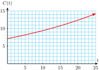
The functions in Investigation 4.1 describe exponential growth. During each time interval of a fixed length, the population is multiplied by a certain constant amount. In Part A, the bacteria population grows by a factor of \(3\) every day.
For this reason, we say that \(3\) is the growth factor for the function. Functions that describe exponential growth can be expressed in a standard form.
The initial value of the population was \(P_0 = 300\text{,}\) and its weekly growth factor is \(b = 2\text{.}\) Thus, a formula for the population after \(t\) weeks is
The variable \(t\) is given in months, so to write the growth formula for this population, we divide the value of \(t\) by \(3.\) The value of \(t/3\) gives us the number of doubling periods.
Now we need some algebra to see the growth factor for the function. We use the third law of exponents to write \(2^{t/3}\) in another form. Recall that to raise a power to a power, we multiply exponents, so
The initial value of the function is \(P_0 = 60\text{,}\) and the growth factor is \(b = 2^{1/3}\text{,}\) or approximately \(1.26\text{.}\) The rabbit population grows by a factor of about \(1.26\) every month.
A lab technician compares the growth of \(2\) species of bacteria. She starts \(2\) colonies of \(50\) bacteria each. Species A doubles in population every \(2\) days, and species B triples every \(3\) days. Find the growth factor for each species.
Exponential growth occurs in other circumstances, too. For example, if the interest on a savings account is compounded annually, the amount of money in the account grows exponentially.
The amount, $105, becomes the new principal for the second year. To find the amount at the end of the second year, we apply the formula again, with \(P = 105\text{.}\)
Observe that to find the amount at the end of each year, we multiply the principal by a factor of \(1 + r = 1.05\text{.}\) Thus, we can express the amount at the end of the second year as
At the end of each year, we multiply the old balance by another factor of \(1.05\) to get the new amount. We organize our results into a table, where \(A(t)\) represents the amount of money in the account after \(t\) years. For this example, a formula for the amount after \(t\) years is
In general, for an initial investment of \(P\) dollars at an interest rate \(r\) compounded annually, we have the following formula for the amount accumulated after \(t\) years.
\begin{equation*}
\begin{aligned}[t]
\amp P \amp\amp \text{is the principal invested,} \\
\amp r \amp\amp \text{is the interest rate,} \\
\amp t \amp\amp \text{is the time period, in years.}
\end{aligned}
\end{equation*}
The notion of percent increase is often used to describe the growth factor for quantities that grow exponentially. Note carefully the distinction between the percent increase, \(r\text{,}\) and the growth factor, \(b=1+r\text{.}\)
During a period of rapid inflation, prices rose by \(12\)% over \(6\) months. At the beginning of the inflationary period, a pound of butter cost $\(2\text{.}\)
The percent increase in the price of butter is \(12\)% every \(6\) months. Therefore, the growth factor for the price of butter is \(1 + 0.12 = 1.12\) every half-year. If \(P(t)\) represents the price of butter after \(t\) years, then \(P(0) = 2\text{,}\) and every half-year we multiply the price by \(1.12\text{,}\) as shown in the table.
Look closely at the second column of the table. After \(t\) years of inflation, the original price of $\(2\) has been multiplied by \(2t\) factors of \(1.12\text{.}\) Thus,
\begin{equation*}
P = 2(1.12)^{2t}
\end{equation*}
for several values, as shown in the table below. We plot the points and connect them with a smooth curve to obtain the graph shown in the figure at right below.
In the preceding examples, exponential growth was modeled by increasing functions of the form
\begin{equation*}
P(t) = P_0 b^t
\end{equation*}
where \(b \gt 1\text{.}\) The function \(P(t) = P_0b^t\) is a decreasing function if \(0 \lt b \lt 1\text{.}\) In this case, we say that the function describes exponential decay, and the constant \(b\) is called the decay factor. In Investigation 4.15, we consider two examples of exponential decay.
A small coal-mining town has been losing population since 1940, when 5000 people lived there. At each census thereafter (taken at 10-year intervals), the population declined to approximately 0.90 of its earlier figure.
Hint: Express the values you calculated in part (1) using powers of \(0.90\text{.}\) Do you see a connection between the value of \(t\) and the exponent on \(0.90\text{?}\)
Graph your function from part (3) using a calculator. (Use the table to choose an appropriate domain and range.) The graph should resemble your hand-drawn graph from part (2).
A plastic window coating \(1\) millimeter thick decreases the light coming through a window by \(25\)%. This means that \(75\)% of the original amount of light comes through \(1\) millimeter of the coating. Each additional millimeter of coating reduces the light by another \(25\)%.
Hint: Express the values you calculated in part (1) using powers of \(0.75\text{.}\) Do you see a connection between the value of \(x\) and the exponent on \(0.75\text{?}\)
Graph your function from part (3) using a calculator. (Use your table of values to choose an appropriate domain and range.) The graph should resemble your hand-drawn graph from part (2).
Evaluate your function to find the percent of the light that comes through 6 millimeters of plastic coating. What percent comes through \(\dfrac{1}{2}\) millimeter?
Before Example 4.12, we noted that a percent increase of \(r\) (in decimal form) corresponds to a growth factor of \(b = 1 + r\text{.}\) A percent decrease of \(r\) corresponds to a decay factor of \(b = 1 - r\text{.}\) In Part B of Investigation 4.15, each millimeter of plastic reduced the amount of light by \(25\)%, so \(r = 0.25\text{,}\) and the decay factor for the function \(P(x)\) is
\begin{equation*}
\begin{aligned}[t]
b \amp = 1 - r \\
\amp= 1 - 0.25 = 0.75
\end{aligned}
\end{equation*}
David Reed writes in Context magazine: "Computing prices have been falling exponentially—50% every 18 months—for the past 30 years and will probably stay on that curve for another couple of decades." An accounting firm invests $50,000 in new computer equipment.
\(L\) is a linear function with initial value \(5\) and slope \(2\text{;}\)\(E\) is an exponential function with initial value \(5\) and growth factor \(2\text{.}\) In a way, the growth factor of an exponential function is analogous to the slope of a linear function: Each measures how quickly the function is increasing (or decreasing).
However, for each unit increase in \(t\text{,}\)\(2\) units are added to the value of \(L(t)\text{,}\) whereas the value of \(E(t)\) is multiplied by \(2\text{.}\) An exponential function with growth factor \(2\) eventually grows much more rapidly than a linear function with slope \(2\text{,}\) as you can see by comparing the graphs in the figure or the function values in the tables.
A solar energy company sold $\(80,000\) worth of solar collectors last year, its first year of operation. This year its sales rose to $\(88,000\text{,}\) an increase of \(10\)%. The marketing department must estimate its projected sales for the next \(3\) years.
If the marketing department predicts that sales will grow linearly, what should it expect the sales total to be next year? Graph the projected sales figures over the next \(3\) years, assuming that sales will grow linearly.
If the marketing department predicts that sales will grow exponentially, what should it expect the sales total to be next year? Graph the projected sales figures over the next \(3\) years, assuming that sales will grow exponentially.
Let \(L(t)\) represent the company’s total sales \(t\) years after starting business, where \(t = 0\) is the first year of operation. If sales grow linearly, then \(L(t)\) has the form \(L(t) = b + mt.\) Now \(L(0) = 80,000\text{,}\) so the intercept \(b\) is \(80,000\text{.}\) The slope \(m\) of the graph is
where \(\Delta S = 8000\) is the increase in sales during the first year. Thus, \(L(t) = 80,000 + 8000t,\) and sales grow by adding $\(8000\) each year. The expected sales total for the next year is
Let \(E(t)\) represent the company’s sales assuming that sales will grow exponentially. Then \(E(t)\) has the form \(E(t) = E_0b^t\) . The percent increase in sales over the first year was \(r = 0.10\text{,}\) so the growth rate is
\begin{equation*}
b = 1 + r = 1.10
\end{equation*}
The initial value, \(E_0\text{,}\) is \(80,000\text{.}\) Thus, \(E(t) = 80,000(1.10)^t\text{,}\) and sales grow by being multiplied each year by \(1.10\text{.}\) The expected sales total for the next year is
A new car begins to depreciate in value as soon as you drive it off the lot. Some models depreciate linearly, and others depreciate exponentially. Suppose you buy a new car for $20,000, and \(1\) year later its value has decreased to $17,000.
If a quantity is multiplied by a constant factor, \(b\text{,}\) in each time period, we say that it undergoes exponential growth or decay. The constant \(b\) is called the growth factor if \(b\gt 1\) and the decay factor if \(0 \lt b \lt 1\text{.}\)
In linear growth, a constant amount is added to the output for each unit increase in the input. In exponential growth, the output is multiplied by a constant factor for each unit increase in the input.
The computer you want cost $\(1200\) when it first came on the market, but after \(3\) months the price was reduced by \(15\%\text{.}\) What was the price then?
The value of your stock portfolio fell \(10\%\) last year, but this year it increased by \(10\%\text{.}\) How does the current value of your portfolio compare to what it was two years ago?
You got a \(5\%\) raise in January, but then in March everyone took a pay cut of \(5\%\text{.}\) How does your new salary compare to what it was last December?
Write a formula for the value of the car if it has a constant depreciation factor of \(0.70\) per year. What is the value of the car after \(4\) years?
A typical beehive contains \(20,000\) insects. The population can increase in size by a factor of \(2.5\) every \(6\) weeks. How many bees could there be after \(4\) weeks? After \(20\) weeks?
A rancher who started with \(800\) head of cattle finds that his herd increases by a factor of \(1.8\) every \(3\) years. How many head of cattle will he have after \(1\) year? After \(10\) years?
A sum of $\(4000\) is invested in an account that pays \(8\%\) interest compounded annually. How much is in the account after \(2\) years? After \(10\) years?
Otto invests $\(600\) in an account that pays \(7.3\%\) interest compounded annually. How much is in Otto’s account after \(3\) years? After \(6\) years?
Paul bought a house for $\(200,000\) in \(2003\text{.}\) Since \(2003\text{,}\) housing prices have risen an average of \(5\%\) per year. How much was the house worth in \(2015\text{?}\) How much will it be worth in 2030?
Sales of Windsurfers have increased \(12\%\) per year since \(2010\text{.}\) If Sunsails sold \(1500\) Windsurfers in \(2010\text{,}\) how many did it sell in \(2015\text{?}\) How many should it expect to sell in \(2022\text{?}\)
During a vigorous spraying program, the mosquito population was reduced to \(\dfrac{3}{4} \) of its previous size every \(2\) weeks. If the mosquito population was originally estimated at \(250,000\text{,}\) how many mosquitoes remained after \(3\) weeks of spraying? After \(8\) weeks?
The number of perch in Hidden Lake has declined to half of its previous value every \(5\) years since 1985, when the perch population was estimated at \(8000\text{.}\) How many perch were there in 1995? In 2013?
Scuba divers find that the water in Emerald Lake filters out \(15\%\) of the sunlight for each \(4\) feet that they descend. How much sunlight penetrates to a depth of \(20\) feet? To a depth of \(45\) feet?
Arch’s motorboat cost $\(15,000\) in \(2005\) and has depreciated by \(10\%\) every \(3\) years. How much was the boat worth in \(2014\text{?}\) In \(2015\text{?}\)
Plutonium-238 is a radioactive element that decays over time into a less harmful element at a rate of \(0.8\%\) per year. A power plant has \(50\) pounds of plutonium-238 to dispose of. How much plutonium-238 will be left after \(10\) years? After \(100\) years?
Iodine-131 is a radioactive element that decays at a rate of \(8.3\%\) per day. How much of a \(12\)-gram sample will be left after \(1\) week? After \(15\) days?
Riverside County is the fastest growing county in California. In \(2000\text{,}\) the population was \(1,545,387\text{.}\) Write a formula for the population of Riverside County. (You do not know the value of the growth factor, \(b\text{,}\) yet.)
In \(2004\text{,}\) the population had grown to \(1,871,950\text{.}\) Find the growth factor and the percent rate of growth, rounded to the nearest tenth of a percent.
In \(2006\text{,}\) a new Ford Focus cost \(\$15,574\text{.}\) The value of a Focus decreases exponentially over time. Write a formula for the value of a Focus. (You do not know the value of the decay factor, \(b\text{,}\) yet.)
A \(2\)-year old Focus cost \(\$11,788\text{.}\) Find the decay factor and the percent rate of depreciation, rounded to the nearest tenth of a percent.
In the 1940s, David Lack undertook a study of the European robin. He tagged \(130\) one-year-old robins and found that on average \(35.6\%\) of the birds survived each year. (Source: Burton, 1998)
According to the data, how many robins would have originally hatched to produce \(130\) one-year-olds?
Many insects grow by discrete amounts each time they shed their exoskeletons. Dyar’s rule says that the size of the insect increases by a constant ratio at each stage. (Source: Burton, 1998)
Dyar measured the width of the head of a caterpillar of a swallowtail butterfly at each stage. The caterpillar’s head was initially approximately \(42\) millimeters wide, and \(63.84\) millimeters wide after its first stage. Find the growth ratio.
Francine says that if a population grew by \(48\%\) in \(6\) years, then it grew by \(8\%\) per year. Is she correct? Either justify or correct her calculation.
Delbert says that if a population decreased by \(60\%\) in 5 years, then it decreased by \(12\%\) per year. Is he correct? Either justify or correct his calculation.
The population of the state of Texas was \(16,986,335\) in \(1990\text{.}\) Write a formula in terms of \(r\) for the population of Texas \(t\) years later.
In \(2000\text{,}\) the population was \(20,851,820\text{.}\) Write an equation and solve for \(r\text{.}\) What was the annual percent increase to the nearest hundredth of a percent?
The population of the state of Florida was \(12,937,926\) in \(1990\text{.}\) Write a formula in terms of \(r\) for the population of Florida \(t\) years later.
In \(2000\text{,}\) the population was \(15,982,378\text{.}\) Write an equation and solve for \(r\text{.}\) What was the annual percent increase to the nearest hundredth of a percent?
The population of Rainville was \(10,000\) in \(1990\) and doubled in \(20\) years. What was the annual percent increase to the nearest hundredth percent?
The population of Elmira was \(350,000\) in \(1990\) and doubled in \(20\) years. What was the annual percent increase to the nearest hundredth of a percent?
The population of Boomtown was \(300\) in \(1908\) and tripled in \(7\) years. What was the annual percent increase to the nearest hundredth of a percent?
The population of Fairview was \(15,000\) in \(1962\) and tripled in \(7\) years. What was the annual percent increase to the nearest hundredth of a percent?
A researcher starts 2 populations of fruit flies of different species, each with \(30\) flies. Species A increases by \(30\%\) in \(6\) days and species B increases by \(20\%\) in \(4\) days.
What was the population of species A after \(6\) days? Find the daily growth factor for species A.
A biologist isolates two strains of a particular virus and monitors the growth of each, starting with samples of \(0.01\) gram. Strain A increases by \(10\%\) in \(8\) hours and strain B increases by \(12\%\) in \(9\) hours.
How much did the sample of strain A weigh after \(8\) hours? What was its hourly growth factor?
At a large university \(3\) students start a rumor that final exams have been canceled. After \(2\) hours, \(6\) students (including the first \(3\)) have heard the rumor.
Assuming that the rumor grows linearly, complete the table below for \(L(t)\text{,}\) the number of students who have heard the rumor after \(t\) hours. Then write a formula for the function \(L(t)\text{.}\) Graph the function.
Complete the table below, assuming that the rumor grows exponentially. Write a formula for the function \(E(t)\) and graph it on the same set of axes with \(L(t)\text{.}\)
Over the weekend the Midland Infirmary identifies four cases of Asian flu. Three days later it has treated a total of ten cases.
Assuming that the number of flu cases grows linearly, complete the table below for \(L(t)\text{,}\) the number of people infected after \(t\) days. Then write a formula for the function \(L(t)\text{.}\) Graph the function.
Complete the table below, assuming that the flu grows exponentially. Write a formula for the function \(E(t)\) and graph it on the same set of axes with \(L(t)\text{.}\)
In 2003, the Center for Biological Diversity filed a lawsuit against the federal government for failing to protect Alaskan sea otters. The population of sea otters, which numbered between 150,000 and 300,000 before hunting began in 1741, declined from about 20,000 in 1992 to 6000 in 2000. (Source: Center for Biological Diversity)
If the population declined linearly after 1992, what was its annual rate of change in population?