Logo image

Modeling, Functions, and Graphs

Section 8.3 Solving Linear Systems Using Matrices

In this section, we consider a mathematical tool called a matrix (plural: matrices) that has wide application in mathematics, business, science, and engineering. A matrix is a rectangular array of numbers or entries. These entries are ordinarily displayed in rows and columns, and the entire matrix is enclosed in brackets or parentheses. Thus,
\begin{equation*} \begin{bmatrix}1\amp 2\amp 3 \\ 4 \amp5 \amp6 \\ 7 \amp8\amp 9 \end{bmatrix}, \begin{bmatrix}2\amp -1\amp 3 \\4\amp 0\amp 2 \end{bmatrix}, \text{ and } \begin{bmatrix} 4\\5\\6 \end{bmatrix} \end{equation*}
are matrices. A matrix of order, or dimension, \(n\times m\) (read "\(n\) by \(m\)") has \(n\) (horizontal) rows and \(m\) (vertical) columns.
The matrices above are \(3\times 3\text{,}\) \(2\times 3\text{,}\) and \(3\times 1\text{,}\) respectively. The first matrix—in which the number of rows is equal to the number of columns—is an example of a square matrix.

Subsection Coefficient Matrix and Augmented Matrix of a System

We will use matrices to solve systems of linear equations. For a system of linear equations of the form
\begin{align*} a_1 x + b_1 y + c_1 z \amp= d_1\\ a_2 x + b_2 y + c_2 z \amp= d_2\\ a_3 x + b_3 y + c_3 z \amp= d_3 \end{align*}
the matrices
\begin{equation*} \begin{bmatrix} a_1\amp b_1\amp c_1 \\ a_2 \amp b_2 \amp c_2 \\ a_3 \amp b_3\amp c_3 \end{bmatrix} \text{ and } \left[ \begin{array}{@{}ccc|c@{}} a_1\amp b_1\amp c_1 \amp d_1\\ a_2 \amp b_2 \amp c_2 \amp d_2\\ a_3 \amp b_3\amp c_3 \amp d_3 \end{array}\right] \end{equation*}
are called the coefficient matrix and the augmented matrix, respectively. Each row of the augmented matrix represents one of the equations of the system. For example, the augmented matrix of the system
\begin{alignat*}{4} 3x\amp {}-{}\amp 4y\amp {}+{}\amp z\amp =\amp 2\\ -x\amp {}+{}\amp 2y\amp \amp \amp =\amp -1\\ 2x\amp {}-{}\amp y\amp {}-{}\amp 3z\amp =\amp 4 \end{alignat*}
is
\begin{equation*} \left[ \begin{array}{@{}ccc|c@{}} 3\amp -4\amp 1 \amp 2\\ -1 \amp 2 \amp 0 \amp -1\\ 2 \amp -1\amp 3 \amp 4 \end{array}\right] \end{equation*}
and the augmented matrix of the system
\begin{alignat*}{4} x\amp {}-{}\amp 3y\amp {}+{}\amp 2z\amp = {}\amp 5\\ \amp {}{}\amp 2y\amp {}-{}\amp z \amp = \amp 4\\ \amp {}{}\amp \amp {}{}\amp 4z\amp = \amp 8 \end{alignat*}
is
\begin{equation*} \left[ \begin{array}{@{}ccc|c@{}} 1\amp -3\amp 2 \amp 5\\ 0 \amp 2 \amp -1 \amp 4\\ 0 \amp 0\amp 4 \amp 8 \end{array}\right] \end{equation*}
The augmented matrix of this last system, which has all zero entries in the lower left corner (below the diagonal), is said to be in upper triangular form. As we saw in Section 8.2, it is easy to find the solution of such a system by back-substitution.

Checkpoint 8.44. Pause and Reflect.

What is the difference between a coefficient matrix and an augmented matrix?

Subsection Elementary Row Operations

The method of elimination depends on two properties of linear systems that allow us to change one system into an equivalent one, that is, one that has the same solutions as the original system.

Properties of Linear Systems.

  1. Multiplying a linear equation by a (nonzero) constant does not change its solutions. That is, any solution of the equation
    \begin{equation*} ax + by = c \end{equation*}
    is also a solution of the equation
    \begin{equation*} kax + kby = kc \end{equation*}
  2. Adding (or subtracting) two linear equations does not change their common solutions. That is, any solution of the system
    \begin{align*} a_1 x + b_1 y \amp = c_1\\ a_2 x + b_2 y \amp = c_2 \end{align*}
    is also a solution of the equation
    \begin{equation*} (a_1 + a_2)x + (b_1 + b_2)y = c_1 + c_2 \end{equation*}
These properties apply to linear systems of any size. Thus, we can perform the following operations on the equations of a system:
  1. Multiply both sides of an equation by a nonzero real number.
  2. Add a constant multiple of one equation to another equation.
  3. Interchange two equations.
Because each equation of the system corresponds to a row in the augmented matrix, the three operations above correspond to three elementary row operations for the augmented matrix. We can perform one or more of these operations on a matrix without changing the solution of the system it represents.

Elementary Row Operations.

  1. Multiply the entries of any row by a nonzero real number.
  2. Add a constant multiple of one row to another row.
  3. Interchange two rows.

Checkpoint 8.45. QuickCheck 1.

Which of the following is not an allowed row operation?
  • A) Divide the entries in a row by a nonzero number
  • B) Add two rows together
  • C) Interchange two elements in a row
  • D) Interchange the first and last rows
Answer.
\(\text{C) Interchange ... in a row}\)
Solution.
Interchange two elements in a row

Example 8.46.

  1. \(A= \left[ \begin{array}{@{}ccc|c@{}} 1 \amp 3 \amp -1 \amp -1\\ 2 \amp 1 \amp 4 \amp 5 \\ 6 \amp 2 \amp -1 \amp -12 \end{array}\right] ~~\) and \(~~B= \left[ \begin{array}{@{}ccc|c@{}} 1 \amp 3 \amp -1 \amp -1\\ 6 \amp 3 \amp 12 \amp 15 \\ 6 \amp 2 \amp -1 \amp -12 \end{array}\right] \)
    represent equivalent systems because we can multiply each entry in the second row of \(A\) by \(3\) to obtain \(B\text{.}\)
  2. \(A= \left[ \begin{array}{@{}ccc|c@{}} 3 \amp -1 \amp 2 \amp 7 \\ 2 \amp 1 \amp 4 \amp -5 \\ 3 \amp 1 \amp 9 \amp -16 \end{array}\right] ~~\) and \(~~B= \left[ \begin{array}{@{}ccc|c@{}} 3 \amp 1 \amp 9 \amp -16 \\ 2 \amp 1 \amp 4 \amp -5 \\ 3 \amp -1 \amp 2 \amp 7 \end{array}\right] \)
    represent equivalent systems because we can interchange the first and third rows of \(A\) to obtain \(B\text{.}\)
  3. \(A= \left[ \begin{array}{@{}ccc|c@{}} 1 \amp 2 \amp 1 \amp -3 \\ 2 \amp 0 \amp -1\amp 7 \\ 3 \amp 1 \amp 2 \amp 10 \end{array}\right] ~~\) and \(~~B= \left[ \begin{array}{@{}ccc|c@{}} 1 \amp 2 \amp 1 \amp -3 \\ 0 \amp -4 \amp -3\amp 13 \\ 3 \amp 1 \amp 2 \amp 10 \end{array}\right] \)
    represent equivalent systems becausewe can add \(-2\) times each entry of the first row of \(A\) to the corresponding entry of the second row of \(A\) to obtain \(B\text{.}\)

Checkpoint 8.47. Practice 1.

Subtract \(4\) times row 2 from row 3.
\begin{equation*} \left[ \begin{array}{@{}ccc|c@{}} 3 \amp 2 \amp -5 \amp -3 \\ 2 \amp -3 \amp 2 \amp 6 \\ 8 \amp -4 \amp 2 \amp 12 \end{array}\right] \end{equation*}
The new row 3 becomes
\({\Large[ ~ }\) \(\big|\) \({\Large]}\)
Answer 1.
\(0\)
Answer 2.
\(8\)
Answer 3.
\(-6\)
Answer 4.
\(-12\)
Solution.
\(\left[ \begin{array}{@{}ccc|c@{}} 3 \amp 2 \amp -5 \amp -3 \\ 2 \amp -3 \amp 2 \amp 6 \\ 0 \amp 8 \amp -6 \amp -12 \end{array}\right]\)

Example 8.48.

Use row operations to form an equivalent matrix with the given elements:
\begin{equation*} \left[ \begin{array}{@{}cc|c@{}} 1 \amp -4 \amp -5 \\ 3 \amp 6 \amp 3\\ \end{array}\right] \longrightarrow \left[ \begin{array}{@{}cc|c@{}} 1 \amp -4 \amp -5 \\ 0 \amp \text{?} \amp \text{?} \\ \end{array}\right] \end{equation*}
Solution.
To obtain \(0\) as the first entry in the second row, we can multiply the first row by \(-3\) and add the result to the second row. That is, we add \(-3(\text{row }1)\) to \(\text{row }2\text{:}\)
\begin{equation*} \left[ \begin{array}{@{}cc|c@{}} 1 \amp -4 \amp -5 \\ 3 \amp 6 \amp 3\\ \end{array}\right] \xrightarrow[\blert{-3(\text{row } 1) + \text{row }2}]{} \left[ \begin{array}{@{}cc|c@{}} 1 \amp -4 \amp -5 \\ 0 \amp 18 \amp 18 \\ \end{array}\right] \end{equation*}

Checkpoint 8.49. Practice 2.

Use row operations to form an equivalent matrix with the given elements:
\begin{equation*} \left[ \begin{array}{@{}cc|c@{}} 1 \amp -3 \amp 7 \\ -2 \amp 4 \amp -6\\ \end{array}\right] \longrightarrow \left[ \begin{array}{@{}cc|c@{}} 1 \amp -3 \amp 7 \\ 0 \amp \text{?} \amp \text{?} \\ \end{array}\right] \end{equation*}
We add times row 1 to row 2.
The new row 2 becomes
\({\Large[ ~ } 0\) \(\big|\) \(\Large]\)
Answer 1.
\(2\)
Answer 2.
\(-2\)
Answer 3.
\(8\)
Solution.
\(\blert{2(\text{row }1)+\text{row }2:} \left[ \begin{array}{@{}cc|c@{}} 1 \amp -3 \amp 7 \\ 0 \amp -2 \amp 8 \\ \end{array}\right]\)

Example 8.50.

Use row operations on the first matrix to form an equivalent matrix in upper triangular form.
\begin{equation*} \left[ \begin{array}{@{}ccc|c@{}} 1 \amp -3 \amp 1 \amp -4 \\ 3 \amp -1 \amp -1 \amp 8\\ 2 \amp -2 \amp 3 \amp -1\\ \end{array}\right] \longrightarrow \left[ \begin{array}{@{}ccc|c@{}} 1 \amp -3 \amp 1 \amp -4 \\ 0 \amp \text{?} \amp \text{?} \amp \text{?} \\ 0 \amp 0 \amp \text{?} \amp \text{?} \\ \end{array}\right] \end{equation*}
Solution.
We perform the transformation in two steps. First, we obtain zeros in the lower two entries of the first column. We get these zeros by adding suitable multiples of the first row to the second and third rows:
\begin{equation*} \left[ \begin{array}{@{}ccc|c@{}} 1 \amp -3 \amp 1 \amp -4 \\ 3 \amp -1 \amp -1 \amp 8\\ 2 \amp -2 \amp 3 \amp -1\\ \end{array}\right] \xrightarrow[\blert{-2(\text{row } 1) + \text{row }3}]{\blert{-3(\text{row } 1) + \text{row }2}} \left[ \begin{array}{@{}ccc|c@{}} 1 \amp -3 \amp 1 \amp -4 \\ 0 \amp 8 \amp -4 \amp 20 \\ 0 \amp 4 \amp 1 \amp 7 \\ \end{array}\right] \end{equation*}
Next we obtain a zero as the second entry of the third row by adding a suitable multiple of the second row. For this matrix, we add \(-12(\text{row }2)\) to \(\text{row }3\text{:}\)
\begin{equation*} \left[ \begin{array}{@{}ccc|c@{}} 1 \amp -3 \amp 1 \amp -4 \\ 0 \amp 8 \amp -4 \amp 20 \\ 0 \amp 4 \amp 1 \amp 7 \\ \end{array}\right] \xrightarrow[\blert{\frac{-1}{2}(\text{row } 2) + \text{row }3}]{} \left[ \begin{array}{@{}ccc|c@{}} 1 \amp -3 \amp 1 \amp -4 \\ 0 \amp 8 \amp -4 \amp 20 \\ 0 \amp 0 \amp 3 \amp -3 \\ \end{array}\right] \end{equation*}
The last matrix is in upper triangular form.

Checkpoint 8.51. Practice 3.

Use the suggested row operations to form an equivalent matrix in upper triangular form.
\begin{equation*} \left[ \begin{array}{@{}ccc|c@{}} 1 \amp -2 \amp 4 \amp 3 \\ 5 \amp -7 \amp 8 \amp 6\\ -2\amp 6 \amp -7 \amp 6\\ \end{array}\right] \longrightarrow \left[ \begin{array}{@{}ccc|c@{}} 1 \amp -2 \amp 4 \amp 3 \\ 0 \amp \text{?} \amp \text{?} \amp \text{?} \\ 0 \amp 0 \amp \text{?} \amp \text{?} \\ \end{array}\right] \end{equation*}
  1. Add \(-5 (\text{row }1)\) to \((\text{row }2)\text{.}\)
    The new row 2 becomes
    \({\Large[ ~ } 0\) \(\big|\) \({\Large]}\)
  2. Add \(2 (\text{row }1)\) to \((\text{row }3)\text{.}\)
    The new row 3 becomes
    \({\Large[ ~ } 0\) \(\big|\) \({\Large]}\)
  3. Multiply \((\text{row }2)\) by \(\dfrac{1}{3}\text{.}\)
    The new row 2 becomes
    \({\Large[ ~ } 0\) \(\big|\) \({\Large]}\)
  4. Add \(-2 (\text{row }2)\) to \((\text{row }3)\text{.}\)
    The new row 3 becomes
    \({\Large[ ~ } 0\) \(\vphantom{{\Large[ ~ }}0\) \(\big|\) \({\Large]}\)
Answer 1.
\(3\)
Answer 2.
\(-12\)
Answer 3.
\(-9\)
Answer 4.
\(2\)
Answer 5.
\(1\)
Answer 6.
\(12\)
Answer 7.
\(1\)
Answer 8.
\(-4\)
Answer 9.
\(-3\)
Answer 10.
\(9\)
Answer 11.
\(18\)
Solution.
\(\left[ \begin{array}{@{}ccc|c@{}} 1 \amp -2 \amp 4 \amp 3 \\ 0 \amp 1 \amp -4 \amp -3 \\ 0 \amp 0 \amp 9 \amp 18 \\ \end{array}\right]\)

Subsection Matrix Reduction

We use elementary row operations to apply Gaussian reduction to the augmented matrix of a linear system. This matrix method can be used to solve linear systems of any size and is well suited for implementation by a computer program. The method has three steps.

Solving a Linear System by Matrix Reduction.

  1. Write the augmented matrix for the system.
  2. Using elementary row operations, transform the matrix into an equivalent one in upper triangular form.
  3. Use back-substitution to find the solution to the system.

Example 8.52.

Use matrix reduction to solve the system.
\begin{alignat*}{3} x\amp {}-{}\amp 2y\amp = {}\amp -5\\ 2x\amp {}+{}\amp 3y\amp = \amp 11 \end{alignat*}
Solution.
The augmented matrix is
\begin{equation*} \left[ \begin{array}{@{}cc|c@{}} 1 \amp -2 \amp -5 \\ 2 \amp 3 \amp 11\\ \end{array}\right] \end{equation*}
We use row operations to obtain \(0\) in the first entry of the second row.
\begin{equation*} \left[ \begin{array}{@{}cc|c@{}} 1 \amp -2 \amp -5 \\ 2 \amp 3 \amp 11\\ \end{array}\right] \xrightarrow[\blert{-2(\text{row } 1) + \text{row }2}]{} \left[ \begin{array}{@{}cc|c@{}} 1 \amp -2 \amp -5 \\ 0 \amp 7 \amp 21 \\ \end{array}\right] \end{equation*}
The last matrix is upper triangular and corresponds to the system
\begin{alignat*}{3} x\amp {}-{}\amp 2y\amp = {}\amp -5\hphantom{blankblank}\amp(1)\\ \amp {}{}\amp 7y\amp = \amp 21\hphantom{blankblank}\amp(2) \end{alignat*}
Now we use back-substitution to solve the system. From Equation (2), \(y=3\text{.}\) Substitute \(3\) for \(y\) in Equation (1) to find
\begin{align*} x - 2(\alert{3}) \amp = -5\\ x \amp = 1 \end{align*}
The solution is the ordered pair \((1, 3)\text{.}\)

Checkpoint 8.53. Practice 4.

Use matrix reduction to solve the system
\begin{equation*} \begin{alignedat}{3} x\amp {}+{}\amp 4y\amp = {}\amp 3\\ 3x\amp {}+{}\amp 8y\amp = \amp 1 \end{alignedat} \end{equation*}
Follow the suggested steps:
  1. Write the augmented matrix for the system.
  2. Add \(-3(\text{row }1)\) to \((\text{row }2)\text{.}\)
  3. Solve the resulting system by back-substitution.
Solution: Give the solution as an ordered pair.
Answer.
\(\left(-5,2\right)\)
Solution.
\((-5, 2)\)

Checkpoint 8.54. Pause and Reflect.

Why do we want to put a matrix into upper triangular form?

Subsection Reducing a \(3\times 3\) Matrix

Although there are many ways to reduce an augmented \(3\times 3\) matrix to upper triangular form, the following two-step procedure may help you organize the row operations.

Strategy for Matrix Reduction.

  1. If the first entry in the first row is zero, interchange that row with another. Obtain zeros in the first entries of the second and third rows by adding suitable multiples of the first row to the second and third rows.
  2. If the second entry of the second row is zero, interchange the second and third rows. Obtain a zero in the second entry of the third row by adding a suitable multiple of the second row to the third row.
If you cannot obtain nonzero entries on the diagonal, then the system does not have a unique solution; the system is either inconsistent or dependent. See Homework Problems 45–48.

Checkpoint 8.55. QuickCheck 2.

What happens if we cannot obtain nonzero entries on the diagonal?
  • A) There is no solution.
  • B) There is no unique solution.
  • C) We should reduce the matrix.
  • D) We should augment the matrix.
Answer.
\(\text{B) There ... unique solution.}\)
Solution.
There is no unique solution.

Example 8.56.

Use matrix reduction to solve the system.
\begin{alignat*}{4} 2x\amp {}-{}\amp 4y\amp {}{}\amp \amp =\amp 6\\ 3x\amp {}-{}\amp 4y\amp {}+{}\amp z \amp =\amp 8\\ 2x\amp {}{}\amp \amp {}-{}\amp 3z\amp =\amp -11 \end{alignat*}
Solution.
The augmented matrix is
\begin{equation*} \left[ \begin{array}{@{}ccc|c@{}} 2 \amp -4\amp 0 \amp 6 \\ 3 \amp -4\amp 1 \amp 8 \\ 2 \amp 0\amp -3 \amp -11 \end{array}\right] \end{equation*}
We obtain \(1\) as the first entry of the first row by multiplying each entry in the first row by \(\dfrac{1}{2}\text{.}\) This will make it easier to obtain zeros in the first entries of the second and third rows.
\begin{equation*} \left[ \begin{array}{@{}ccc|c@{}} 2 \amp -4\amp 0 \amp 6 \\ 3 \amp -4\amp 1 \amp 8 \\ 2 \amp 0\amp -3 \amp -11 \end{array}\right] \end{equation*}
\begin{alignat*}{4} 2x\amp {}-{}\amp 4y\amp {}+{}\amp0z \amp =\amp 6\\ 3x\amp {}-{}\amp 4y\amp {}+{}\amp z \amp =\amp 8\\ 2x\amp {}+{}\amp 0y\amp {}-{}\amp 3z\amp =\amp -11 \end{alignat*}
\begin{equation*} \stackrel{\displaystyle{\frac{1}{2}}(\text{row }1)}{\big\downarrow} \end{equation*}
\begin{equation*} \left[ \begin{array}{@{}ccc|c@{}} 1 \amp -2\amp 0 \amp 3 \\ 3 \amp -4\amp 1 \amp 8 \\ 2 \amp 0\amp -3 \amp -11 \end{array}\right] \end{equation*}
\begin{alignat*}{4} x\amp {}-{}\amp 2y\amp {}+{}\amp 0z \amp =\amp 3\\ 3x\amp {}-{}\amp 4y\amp {}+{}\amp z \amp =\amp 8\\ 2x\amp {}+{}\amp 0y\amp {}-{}\amp 3z\amp =\amp -11 \end{alignat*}
Next, we obtain zeros in the first entries of the second and third rows by adding suitable multiples of the first row:
\begin{equation*} -3(\text{row }1) + 2~~{\Bigg\downarrow}~~3(\text{row }1) + 3 \end{equation*}
\begin{equation*} \left[ \begin{array}{@{}ccc|c@{}} 1 \amp -2\amp 0 \amp 3 \\ 0 \amp 2 \amp 1 \amp -1 \\ 0 \amp 4\amp -3 \amp -17 \end{array}\right] \end{equation*}
\begin{alignat*}{4} x\amp {}-{}\amp 2y\amp {}+{}\amp 0z \amp =\amp 3\\ x\amp {}+{}\amp 2y\amp {}+{}\amp z \amp =\amp -1\\ 0x\amp {}+{}\amp 4y\amp {}-{}\amp 3z\amp =\amp -17 \end{alignat*}
Finally, we obtain a zero in the second entry of the third row by adding \(-2(\text{row }2)\) to \(\text{row }3\text{:}\)
\begin{equation*} -2(\text{row }2) + 3~~{\Bigg\downarrow}~~\hphantom{3(\text{row }1) + 3} \end{equation*}
\begin{equation*} \left[ \begin{array}{@{}ccc|c@{}} 1 \amp -2\amp 0 \amp 3 \\ 0 \amp 2 \amp 1 \amp -1 \\ 0 \amp 0 \amp -5 \amp -15 \end{array}\right] \end{equation*}
\begin{alignat*}{4} x\amp {}-{}\amp 2y\amp {}+{}\amp 0z \amp =\amp 3\\ 0x\amp {}+{}\amp 2y\amp {}+{}\amp z \amp =\amp -1\\ 0x\amp {}+{}\amp 0y\amp {}-{}\amp 5z\amp =\amp -15 \end{alignat*}
The system is now in upper triangular form, and we use back-substitution to find the solution. We solve the last equation to get \(z=3\) and substitute \(3\) for \(z\) in the second equation to find \(y=-2\text{.}\) Finally, we substitute \(3\) for \(z\) and \(-2\) for \(y\) in the first equation to find \(x=-1\text{.}\) The solution is the ordered triple \((-1,-2, 3)\text{.}\)

Checkpoint 8.57. Practice 5.

Use matrix reduction to solve the system
\begin{equation*} \begin{aligned} x + 3z \amp = -11\\ 2x + y + z \amp = 1\\ -3x - 2y = 3 \end{aligned} \end{equation*}
Follow the suggested steps:
  1. Write the augmented matrix for the system.
  2. Add \(-2\)(row 1) to (row 2).
  3. Add \(3\)(row 1) to (row 3).
  4. Add \(2\)(row 2) to (row 3).
  5. Solve the resulting system by back-substitution.
Solution: Give the solution as an ordered triple.
Answer.
\(\left(37,-57,-16\right)\)
Solution.
\((37, -57, -16)\)
It is a good idea to make the first entry in the first row equal to \(1\text{,}\) as we did in Example 8.56, to simplify the calculations that follow. However, if that entry is zero we can interchange two rows. For example, to reduce the matrix
\begin{equation*} \left[ \begin{array}{@{}ccc|c@{}} 0 \amp 1 \amp 2 \amp 3 \\ 1 \amp 2 \amp 3 \amp 4 \\ 2 \amp 5 \amp 1 \amp 4 \end{array}\right] \end{equation*}
we begin by interchanging the first and second rows to obtain
\begin{equation*} \left[ \begin{array}{@{}ccc|c@{}} 1 \amp 2 \amp 3 \amp 4 \\ 0 \amp 1 \amp 2 \amp 3 \\ 2 \amp 5 \amp 1 \amp 4 \end{array}\right] \end{equation*}
We then follow the two-step procedure described above to find
\begin{equation*} \blert{\xrightarrow[-2(\text{row } 1) + \text{row }3]{}} \left[ \begin{array}{@{}ccc|c@{}} 1 \amp 2 \amp 3 \amp 4 \\ 0 \amp 1 \amp 2 \amp 3 \\ 0 \amp 1 \amp -5 \amp -4 \end{array}\right] \blert{\xrightarrow[-(\text{row } 2) + \text{row }3]{}} \left[ \begin{array}{@{}ccc|c@{}} 1 \amp 2 \amp 3 \amp 4 \\ 0 \amp 1 \amp 2 \amp 3 \\ 0 \amp 0 \amp -7 \amp -7 \end{array}\right] \end{equation*}

Checkpoint 8.58. QuickCheck 3.

What should you do if the first entry in the first row is zero?
  • Interchange two columns
  • Interchange two rows
  • Add the first row to the second row
  • Obtain zeros below that entry
Answer.
\(\text{Interchange two rows}\)
Solution.
Interchange two rows

Subsection Solving Larger Systems

Systems of linear equations in business and economics may involve hundreds of linear equations and hundreds of variables. The study of airflow for aircraft design can involve systems of millions of linear equations and variables. These large systems are solved using matrix methods.

Example 8.59.

Write the augmented matrix for the system
\begin{alignat*}{5} -w\amp {}+{} \amp x \amp {}-{}\amp y\amp {}+{}\amp z \amp =\amp 7\\ 2w\amp {}-{}\amp 2x\amp {}-{}\amp 4y\amp {}-{}\amp 5z \amp =\amp -17\\ -3w\amp {}+{}\amp 9x\amp {}+{}\amp 3y\amp {}+{}\amp 6z\amp =\amp 30\\ 4w\amp {}+{}\amp 8x\amp {}-{}\amp 2y\amp {}+{}\amp 5z\amp =\amp 17 \end{alignat*}
Use matrix reduction and back-substitution to solve the system.
Solution.
The augmented matrix is
\begin{equation*} \left[ \begin{array}{@{}cccc|c@{}} -1 \amp 1 \amp -1 \amp 1 \amp 7 \\ 2 \amp -2 \amp -4 \amp -5 \amp -17 \\ -3 \amp 9 \amp 3 \amp 6 \amp 30 \\ 4 \amp 8 \amp -2 \amp 5 \amp 17 \end{array}\right] \end{equation*}
We use row operations to put the matrix in upper triangular form. First, we add multiples of the first row to the rows below it to get \(0\)s in the first column.
\(~~\)
\(\blert{2(\text{row }1) + \text{row }2}\)
\(\blert{-3(\text{row }1) + \text{row }3}\)
\(\blert{4(\text{row }1) + \text{row }4}\)
\begin{equation*} \left[ \begin{array}{@{}cccc|c@{}} -1 \amp 1 \amp -1 \amp 1 \amp 7 \\ 0 \amp 0 \amp -6 \amp -3 \amp -3 \\ 0 \amp 6 \amp 6 \amp 3 \amp 9 \\ 0 \amp 12 \amp -6 \amp 9 \amp 45 \end{array}\right] \end{equation*}
The second row has \(0\) as its second entry, so we interchange the second and third rows to put a nonzero entry in the second column.
\begin{equation*} \left[ \begin{array}{@{}cccc|c@{}} -1 \amp 1 \amp -1 \amp 1 \amp 7 \\ 0 \amp 6 \amp 6 \amp 3 \amp 9 \\ 0 \amp 0 \amp -6 \amp -3 \amp -3 \\ 0 \amp 12 \amp -6 \amp 9 \amp 45 \end{array}\right] \end{equation*}
Now we want \(0\)s in the last two rows of the second column. The third row already has \(0\) in the second column, so we only need to add a multiple of the second row to the fourth row.
\(~~\)
\(~~\)
\(~~\)
\(\blert{-2(\text{row }2) + \text{row }4}\)
\begin{equation*} \left[ \begin{array}{@{}cccc|c@{}} -1 \amp 1 \amp -1 \amp 1 \amp 7 \\ 0 \amp 6 \amp 6 \amp 3 \amp 9 \\ 0 \amp 0 \amp -6 \amp -3 \amp -3 \\ 0 \amp 0 \amp -18\amp 3 \amp 27 \end{array}\right] \end{equation*}
Finally, we add a multiple of the third row to the fourth row to get 0 in the third column.
\(~~\)
\(~~\)
\(~~\)
\(\blert{-3(\text{row }3) + \text{row }4}\)
\begin{equation*} \left[ \begin{array}{@{}cccc|c@{}} -1 \amp 1 \amp -1 \amp 1 \amp 7 \\ 0 \amp 6 \amp 6 \amp 3 \amp 9 \\ 0 \amp 0 \amp -6 \amp -3 \amp -3 \\ 0 \amp 0 \amp 0 \amp 12 \amp 36 \end{array}\right] \end{equation*}
This triangular matrix corresponds to the system
\begin{alignat*}{5} -w\amp {}+{} \amp x \amp {}-{}\amp y\amp {}+{}\amp z \amp =\amp 7\\ \amp {} {}\amp 6x\amp {}+{}\amp 6y\amp {}+{}\amp 3z \amp =\amp 9\\ \amp {}{}\amp \amp {} {}\amp 6y\amp {}+{}\amp 3z\amp =\amp -3\\ \amp {} {}\amp \amp {} {}\amp \amp {} {}\amp 12z\amp =\amp 36 \end{alignat*}
which we solve by back-substitution.
From the last equation, we find \(z=3\text{,}\) and by substituting \(3\) for \(z\) in the third equation, we find \(y=-1\text{.}\) Next, we substitute \(-1\) for \(y\) and \(3\) for \(z\) in the second equation to find \(x=1\text{,}\) and finally, we substitute \(x=1\text{,}\) \(y=-1\text{,}\) \(z=3\) into the first equation to find \(w=-2\text{.}\)
The solution is the ordered four-tuple \((-2, 1, -1, 3)\text{.}\) We can verify that these values satisfy all four equations of the original system.
Our strategy for reducing \(3\times 4\) augmented matrices can be generalized for larger matrices, as demonstrated in Example 8.59. Starting with the first row, we work our way along the diagonal, using row operations to obtain nonzero entries on the diagonal and zeros below the diagonal entry.

Checkpoint 8.60. Practice 6.

Use matrix reduction to solve the system
\begin{equation*} \begin{alignedat}{5} w\amp {}+{} \amp x \amp {}+{}\amp y\amp {}+{}\amp z \amp =\amp -1\\ -w\amp {}+{}\amp x\amp {}-{}\amp y\amp {}+{}\amp z \amp =\amp 3\\ -2w\amp {}+{}\amp 10x\amp {}+{}\amp 4y\amp {}+{}\amp 7z\amp =\amp 23\\ 3w\amp {}+{}\amp 9x\amp {}-{}\amp 3y\amp {}+{}\amp 6z\amp =\amp 0 \end{alignedat} \end{equation*}
Solution: Give the solution as an ordered 4-tuple.
Answer.
\(\left(-3,2,1,-1\right)\)
Solution.
\((-3,2,1,-1)\)

Checkpoint 8.61. Pause and Reflect.

How is matrix reduction similar to Gaussian reduction?

Subsection Reduced Row Echelon Form

The triangular matrix we obtain by row reduction is an example of row echelon form. In a row echelon matrix,
  1. The first nonzero entry in any row is farther to the right than the first nonzero entry in the rows above it.
  2. The entries directly below the first nonzero entry in any row are all zeros.
  3. Any row consisting entirely of zeros is below all rows with any nonzero entry.
If we divide each row by its leading nonzero entry, so that the leading entry is \(1\text{,}\) and if we use row reduction to obtain 0’s above the leading \(1\) as well as below it, the resulting matrix is said to be in reduced row echelon form. This form is especially convenient because we do not have to use back-substitution to finish solving the system; we can read off the solutions directly from the matrix.
For example, you can check that the matrix
\begin{equation*} \left[ \begin{array}{@{}cccc|c@{}} 1 \amp 0 \amp 0 \amp 0 \amp -2 \\ 0 \amp 1 \amp 0 \amp 0 \amp 3 \\ 0 \amp 0 \amp 1 \amp 0 \amp -3 \\ 0 \amp 0 \amp 0 \amp 1 \amp 4 \end{array}\right] \end{equation*}
corresponds to the system
\begin{alignat*}{5} a\amp {}+{} \amp 0b \amp {}+{}\amp 0c\amp {}+{}\amp 0d \amp =\amp -2\\ 0a\amp {}+{}\amp b\amp {}+{}\amp 0c\amp {}+{}\amp 0d \amp =\amp 3\\ 0a\amp {}+{}\amp 0b\amp {}+{}\amp c\amp {}+{}\amp 0d\amp =\amp -3\\ 0a\amp {}+{}\amp 0b\amp {}+{}\amp 0c\amp {}+{}\amp d\amp =\amp 4 \end{alignat*}
From this system, it is easy to read the solutions \(a=-2\text{,}\) \(b=3\text{,}\) \(c=-3\text{,}\) and \(d=4\)

Checkpoint 8.62. QuickCheck 4.

Why is reduced row echelon form useful?
  • A) It makes the elements in each row smaller.
  • B) It lets us read the solutions of a system.
  • C) It reduces the number of rows.
  • D) It solves the matrix.
Answer.
\(\text{B) It ... a system.}\)
Solution.
It lets us read the solutions of a system.

Technology 8.63.

Graphing calculators and other graphing utilitiues typically have a command for finding the reduced row echelon form of a matrix.

Example 8.64.

Solve the system
\begin{alignat*}{5} a\amp {}+{} \amp 2b \amp {}+{}\amp 4c\amp {}+{}\amp 8d \amp =\amp 12\\ -2a\amp {}+{}\amp 2b\amp {}-{}\amp 2c\amp {}+{}\amp 2d \amp =\amp 1\\ 6a\amp {}+{}\amp 6b\amp {}+{}\amp 6c\amp {}+{}\amp 6d\amp =\amp 19\\ 4a\amp {}+{}\amp 20b\amp {}-{}\amp 8c\amp {}+{}\amp 14d\amp =\amp 41 \end{alignat*}
by finding the reduced row echelon form of the augmented matrix.
Solution.
The augmented matrix is
\begin{equation*} \left[ \begin{array}{@{}cccc|c@{}} 1 \amp 2 \amp 4 \amp 8 \amp 12 \\ -2\amp 2 \amp -2\amp 2 \amp 1 \\ 6 \amp 6 \amp 6 \amp 6 \amp 19 \\ 4 \amp 20 \amp -8\amp 14\amp 41 \end{array}\right] \end{equation*}
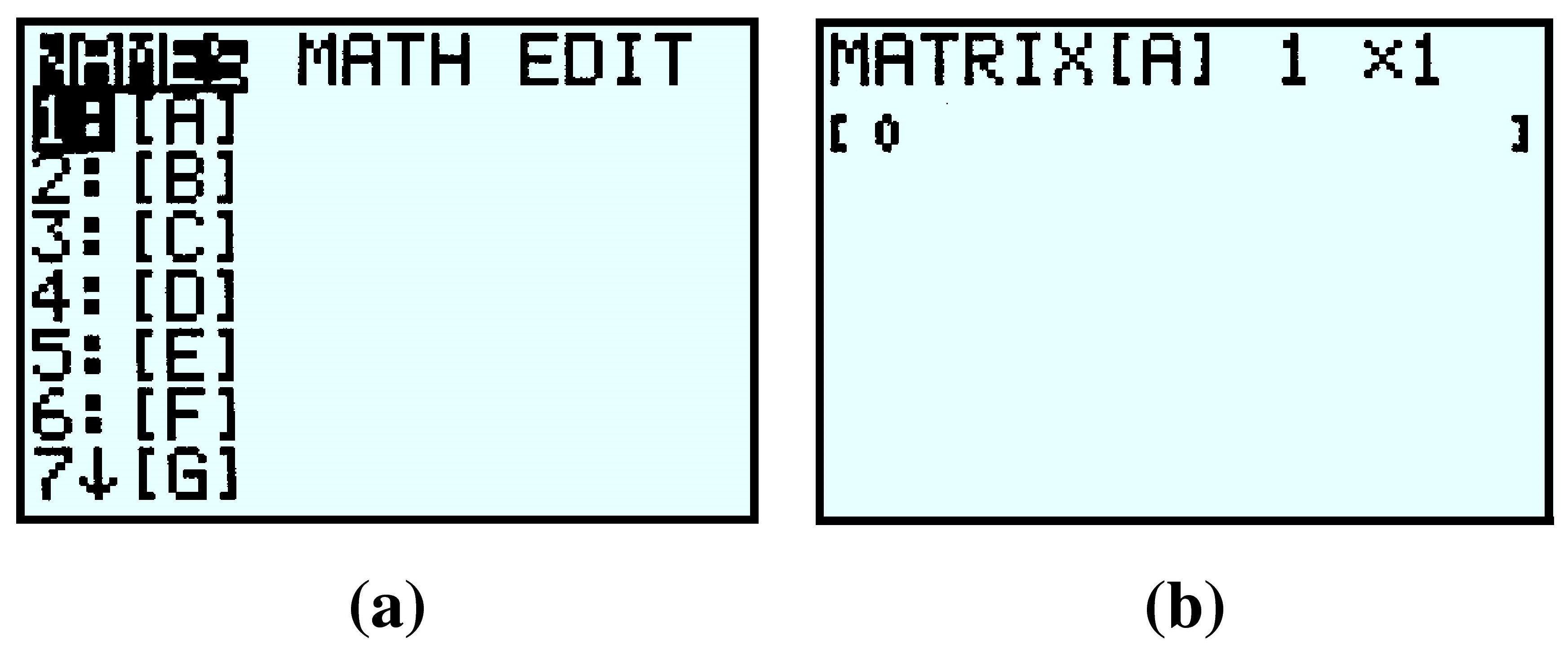
We enter this matrix into the calculator as follows: First access the MATRIX menu by pressing 2nd x^-1 on a TI-84 orMATRX on a TI-83. You will see the menu shown in figure (a). We will use matrix [A], which is already selected, and we presss ENTER to EDIT (or enter) the matrix, shown in figure(b).
GC windows to edit or create a matrix
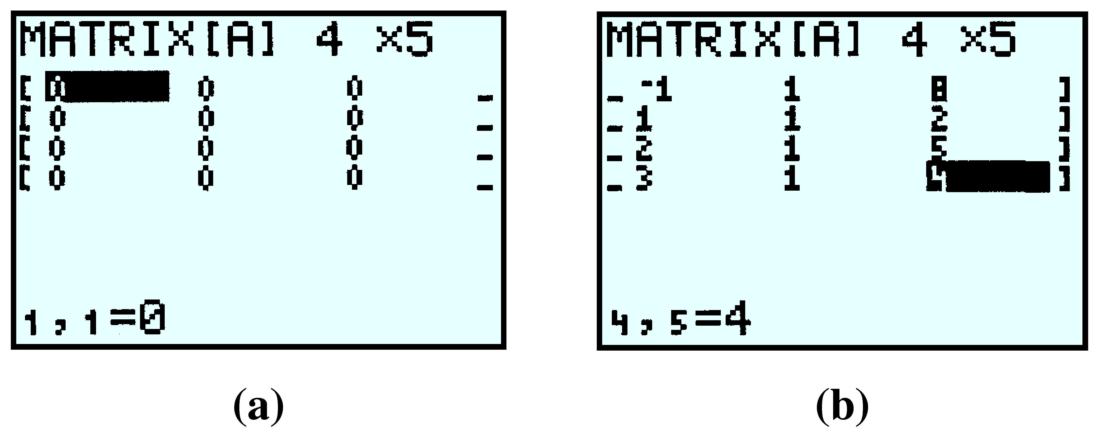
We want to enter a \(4\times 5\) matrix, so we press \(4\)ENTER\(5\)ENTER, and we see the display in figure (a) below. Now type in the first row of the matrix, pressing ENTER after each entry. The calculator automatically moves to the second row. Continue filling in the rest of the augmented matrix, as shown in figure (b).
GC windows of matrices being edited
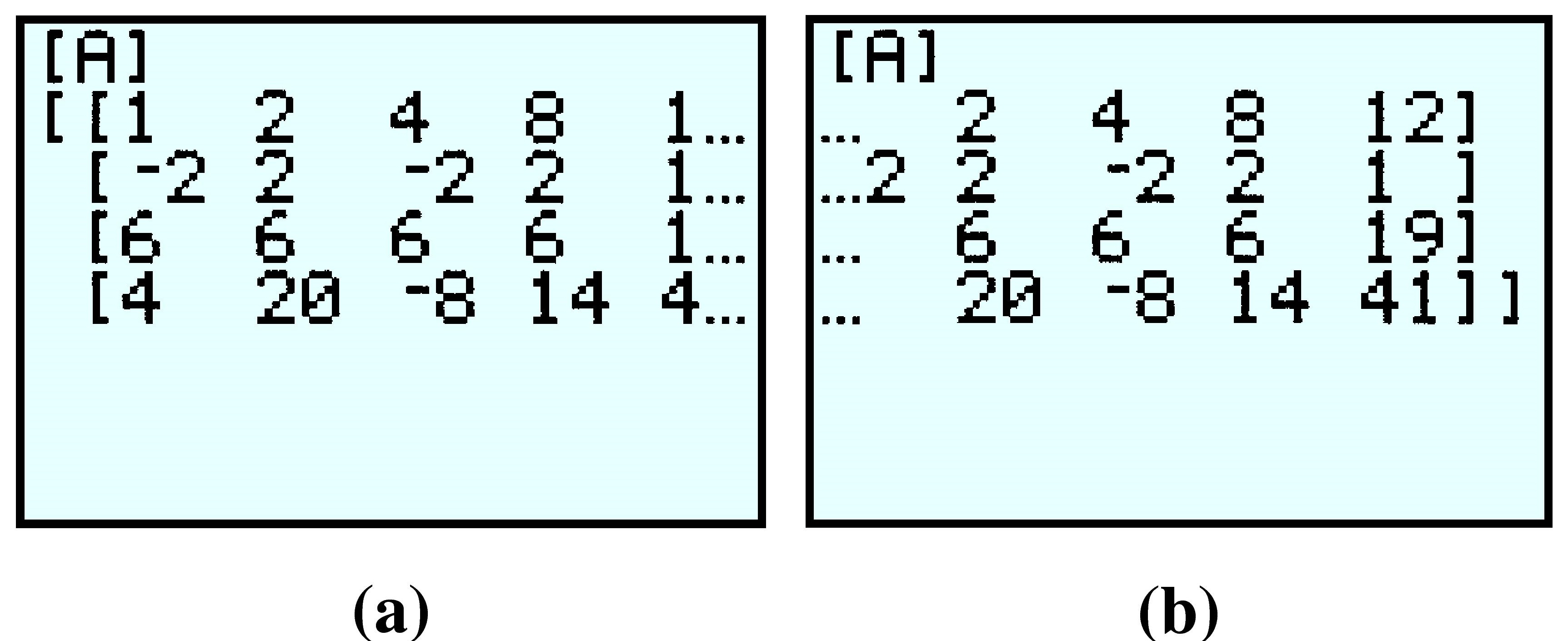
To make sure you have entered the values correctly, press 2ndMODE to quit to the home screen, then open the matrix menu again. Press \(1\)ENTER to retrieve matrix [A]; the calculator display should look like figure (a) below. To check the rest of the matrix, press the right arrow key until you see the last column, as in figure (b).
GC windows scrolling to see a matrix
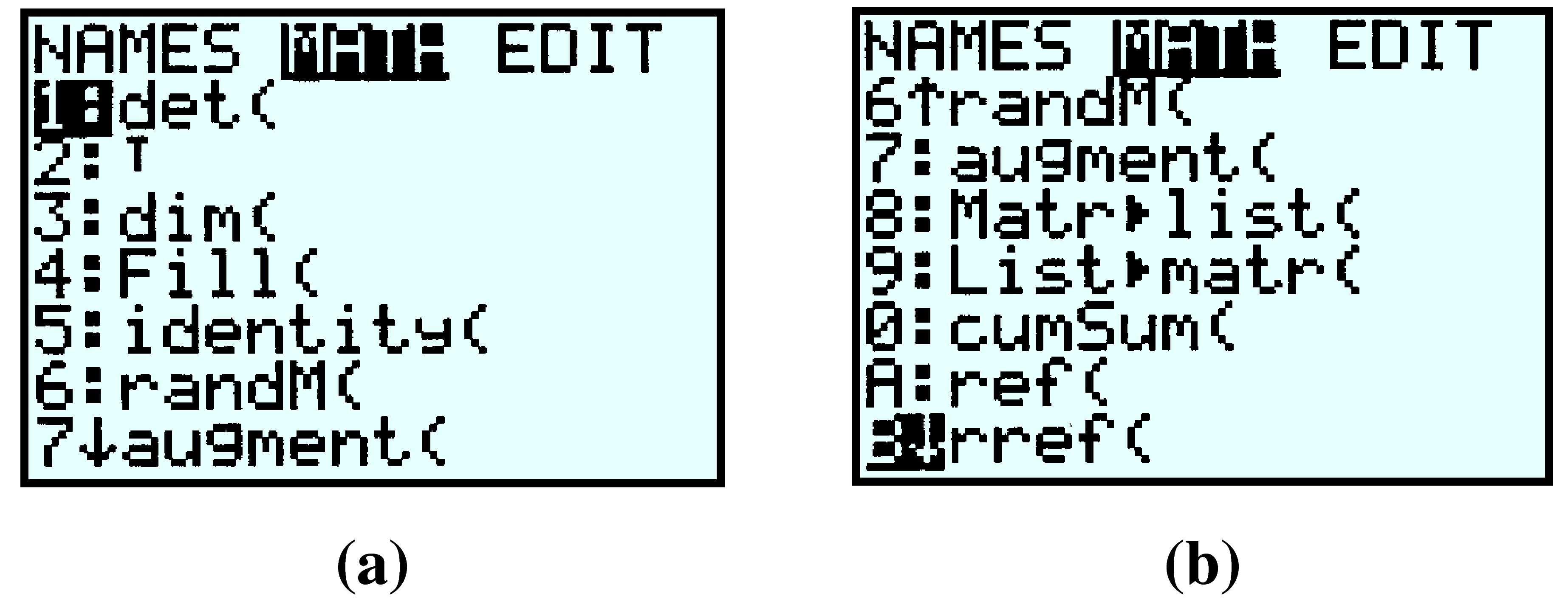
Now we are ready to compute the reduced row echelon form of the matrix. Access the matrix menu again, but this time press the right arrow once to highlight MATH as shown in figure (a). Scroll down until the rref( command is highlighted, as shown in figure (b), and press ENTER.
GC windows to manipulate a matrix
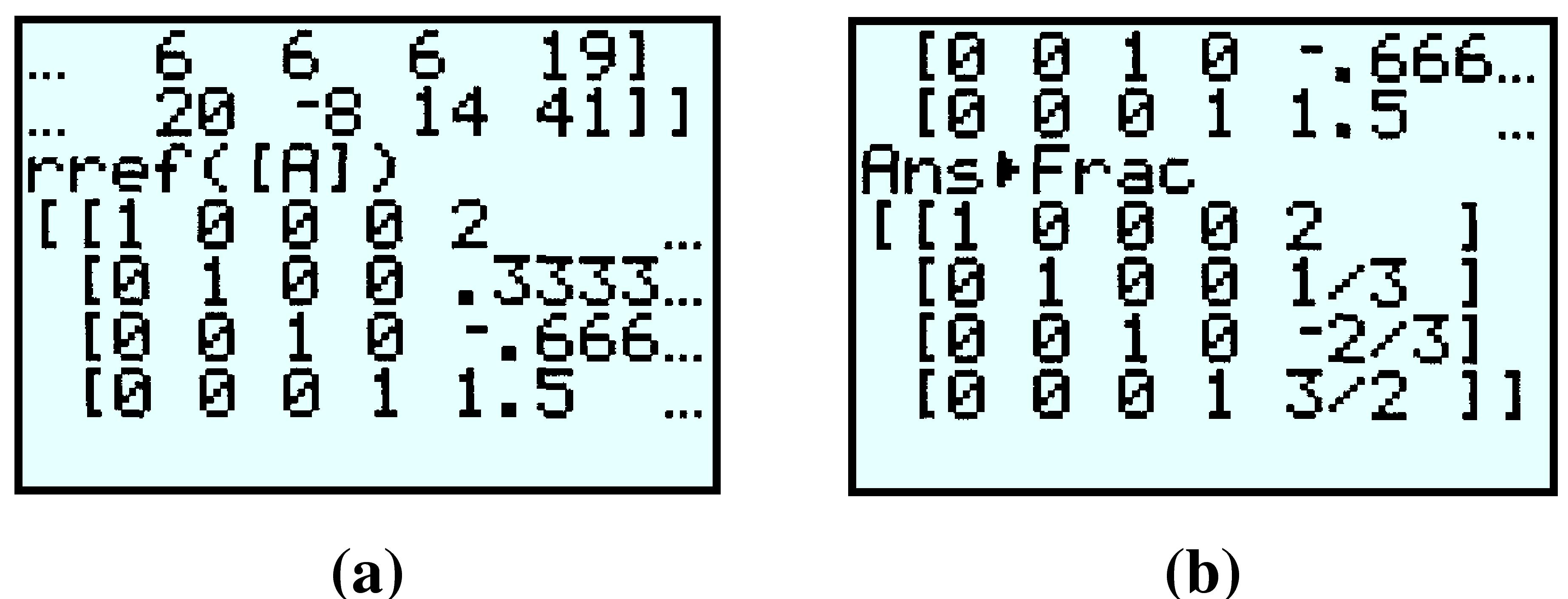
Finally, enter matrix [A] after the rref( command by pressing 2nd x^-1 \(1\)) ENTER or \(MATRX\) \(1\)) ENTER. The display should now look like figure (a) below. The last column of the matrix gives decimal approximations for the solutions.
GC windows showing rref
The calculator can also display the rational form of the solutions: Press MATH ENTER ENTER to see figure(b). The reduced row echelon form of the augmented matrix is thus
\begin{equation*} \left[ \begin{array}{@{}cccc|c@{}} 1 \amp 0 \amp 0 \amp 0 \amp 2 \\ 0 \amp 1 \amp 0 \amp 0 \amp 1/3 \\ 0 \amp 0 \amp 1 \amp 0 \amp -2/3 \\ 0 \amp 0 \amp 0 \amp 1 \amp 3/2 \end{array}\right] \end{equation*}
and the solution is the ordered four-tuple \((2, \dfrac{1}{3}, \dfrac{-2}{3}, \dfrac{3}{2})\text{.}\) You can verify that these values satisfy each of the original four equations.

Checkpoint 8.65. Practice 7.

  1. Find the row reduced echelon form of the augmented matrix for the system
    \begin{equation*} \begin{alignedat}{5} -a\amp {}+{} \amp b \amp {}-{}\amp c\amp {}+{}\amp d \amp =\amp 8\\ a\amp {}+{}\amp b\amp {}+{}\amp c\amp {}+{}\amp d \amp =\amp 2\\ 8a\amp {}+{}\amp 4b\amp {}+{}\amp 2c\amp {}+{}\amp d\amp =\amp 5\\ 27a\amp {}+{}\amp 9b\amp {}-{}\amp 3c\amp {}+{}\amp d\amp =\amp 4 \end{alignedat} \end{equation*}
  2. What third degree polynomial has a graph that passes through the points \((-1, 8)\text{,}\) \((1, 2)\text{,}\) \((2, 5)\text{,}\) and \((3, 4)\text{?}\)
    \(f(x)=\)
Answer.
\(-x^{3}+4x^{2}-2x+1\)
Solution.
  1. \(\displaystyle \)
  2. \(\displaystyle f (x) = -x^3 + 4x^2 - 2x + 1\)

Subsection Section Summary

Subsubsection Vocabulary

Look up the definitions of new terms in the Glossary.
  • Matrix
  • Row echelon form
  • Upper triangular form
  • Coefficient matrix
  • Dimension
  • Entry
  • Reduced row echelon form
  • Elementary row operation
  • Augmented matrix
  • Square matrix
  • Order

Subsubsection CONCEPTS

  1. We can use a matrix to represent a system of linear equations. Each row of the matrix consists of the coefficients in one of the equations of the system.
  2. We operate on a matrix by using the elementary row operations.
    Elementary Row Operations.
    1. Multiply the entries of any row by a nonzero real number.
    2. Add a constant multiple of one row to another row.
    3. Interchange two rows.
  3. We can solve a linear system by matrix reduction.
    Solving a Linear System by Matrix Reduction.
    1. Write the augmented matrix for the system.
    2. Using elementary row operations, transform the matrix into an equivalent one in upper triangular form.
    3. Use back-substitution to find the solution to the system.
  4. Strategy for Matrix Reduction.
    1. If the first entry in the first row is zero, interchange that row with another. Obtain zeros in the first entries of the second and third rows by adding suitable multiples of the first row to the second and third rows.
    2. If the second entry of the second row is zero, interchange the second and third rows. Obtain a zero in the second entry of the third row by adding a suitable multiple of the second row to the third row.
  5. To reduce larger matrices, we start with the first row and work our way along the diagonal, using row operations to obtain nonzero entries on the diagonal and zeros below the diagonal entry.

Subsubsection STUDY QUESTIONS

  1. What are the coefficient matrix and the augmented matrix for a system of equations?
  2. What does it mean for a matrix to be in upper triangular form?
  3. State the three elementary row operations.
  4. Describe a two-step procedure for reducing a \(3\times 3\) matrix to upper triangular form.
  5. Once the matrix is in upper triangular form, how do we complete the solution of the system?
  6. Why is the reduced row echelon form of an augmented matrix convenient for solving a system?

Subsubsection SKILLS

Practice each skill in the Homework problems listed.
  1. Perform elementary row operations: #1–8
  2. Choose an elementry row operation to convert a matrix: #9–18
  3. Solve a system by matrix reduction: #19–34
  4. Solve a system using the reduced row echelon form of the augmented matrix: #35–40

Exercises Homework 8.3

Exercise Group.

Perform the given elementary row operation on the matrices in Problems 1–8.
1.
Multiply \(\text{row }2\) by \(-3\text{:}\)
\begin{equation*} \left[ \begin{array}{@{}cc|c@{}} -2 \amp 1 \amp 0 \\ 3 \amp -1 \amp 2 \end{array}\right] \end{equation*}
2.
Multiply \(\text{row }1\) by \(\dfrac{1}{4} \text{:}\)
\begin{equation*} \left[ \begin{array}{@{}cc|c@{}} 2 \amp 0 \amp 3 \\ -1 \amp 5 \amp 4 \end{array}\right] \end{equation*}
3.
Add \(2(\text{row }1)\) to \(\text{row } 2\text{:}\)
\begin{equation*} \left[ \begin{array}{@{}cc|c@{}} 1 \amp -3 \amp 6 \\ -2 \amp 4 \amp -1 \end{array}\right] \end{equation*}
4.
Add \(-3(\text{row }1)\) to \(\text{row } 2\text{:}\)
\begin{equation*} \left[ \begin{array}{@{}cc|c@{}} 1 \amp -4 \amp 8 \\ 3 \amp -2 \amp 10 \end{array}\right] \end{equation*}
5.
Interchange \(\text{row }1\) and \(\text{row } 3\text{:}\)
\begin{equation*} \left[ \begin{array}{@{}ccc|c@{}} 0 \amp -3 \amp 2 \amp -3 \\ 2 \amp 6 \amp -1 \amp 3 \\ 1 \amp 0 \amp -2 \amp 5 \end{array}\right] \end{equation*}
6.
Interchange \(\text{row }2\) and \(\text{row } 3\text{:}\)
\begin{equation*} \left[ \begin{array}{@{}ccc|c@{}} 1 \amp 6 \amp 0 \amp -2 \\ 0 \amp 0 \amp 5 \amp -10 \\ 0 \amp 3 \amp -2 \amp 8 \end{array}\right] \end{equation*}
7.
Add \(-4(\text{row }1)\) to \(\text{row } 3\text{:}\)
\begin{equation*} \left[ \begin{array}{@{}ccc|c@{}} 1 \amp 2 \amp 1 \amp -5 \\ 0 \amp 4 \amp -2 \amp 3 \\ 4 \amp -1 \amp 6 \amp -8 \end{array}\right] \end{equation*}
8.
Add \(2(\text{row }2)\) to \(\text{row } 3\text{:}\)
\begin{equation*} \left[ \begin{array}{@{}ccc|c@{}} 1 \amp -7 \amp 5 \amp 2 \\ 0 \amp 1 \amp -3 \amp -1 \\ 0 \amp -2 \amp -3 \amp 4 \end{array}\right] \end{equation*}

Exercise Group.

In Problems 9–18, use row operations on the first matrix to form an equivalent matrix with the given entries.
9.
\(\left[ \begin{array}{@{}cc|c@{}} 1 \amp -3 \amp 2 \\ 2 \amp 1 \amp 4\\ \end{array}\right] \longrightarrow \left[ \begin{array}{@{}cc|c@{}} 1 \amp -3 \amp 2 \\ 0 \amp \text{?} \amp \text{?} \\ \end{array}\right] \)
10.
\(\left[ \begin{array}{@{}cc|c@{}} -2 \amp 3 \amp 0 \\ 4 \amp 1 \amp 6 \end{array}\right] \longrightarrow \left[ \begin{array}{@{}cc|c@{}} -2 \amp 3 \amp 0 \\ 0 \amp \text{?} \amp \text{?} \end{array}\right] \)
11.
\(\left[ \begin{array}{@{}cc|c@{}} 2 \amp 6 \amp -4 \\ 5 \amp 3 \amp 1 \end{array}\right] \longrightarrow \left[ \begin{array}{@{}cc|c@{}} 2 \amp 6 \amp -4 \\ \text{?} \amp 0 \amp \text{?} \end{array}\right] \)
12.
\(\left[ \begin{array}{@{}cc|c@{}} 6 \amp 4 \amp -2 \\ -1 \amp -2 \amp -3\\ \end{array}\right] \longrightarrow \left[ \begin{array}{@{}cc|c@{}} 6 \amp 4 \amp -2 \\ \text{?} \amp 0 \amp \text{?} \end{array}\right] \)
13.
\(\left[ \begin{array}{@{}ccc|c@{}} 1 \amp -2 \amp 2 \amp 1 \\ 2 \amp 3 \amp -1 \amp 6 \\ 4 \amp 1 \amp -3 \amp 3 \end{array}\right] \longrightarrow \left[ \begin{array}{@{}ccc|c@{}} 1 \amp -2 \amp 2 \amp 1 \\ 0 \amp \text{?} \amp \text{?} \amp \text{?} \\ 0 \amp \text{?} \amp \text{?} \amp \text{?} \end{array}\right] \)
14.
\(\left[ \begin{array}{@{}ccc|c@{}} 2 \amp -1 \amp 3 \amp -1 \\ -4 \amp 0 \amp 4 \amp 5 \\ 6 \amp 2 \amp -1 \amp -2 \end{array}\right] \longrightarrow \left[ \begin{array}{@{}ccc|c@{}} 2 \amp -1 \amp 3 \amp -1 \\ 0 \amp \text{?} \amp \text{?} \amp \text{?} \\ 0 \amp \text{?} \amp \text{?} \amp \text{?} \end{array}\right] \)
15.
\(\left[ \begin{array}{@{}ccc|c@{}} -1 \amp 4 \amp 3 \amp 2 \\ 2 \amp -2 \amp -4 \amp 6 \\ 1 \amp 2 \amp 3 \amp -3 \end{array}\right] \longrightarrow \left[ \begin{array}{@{}ccc|c@{}} -1 \amp 4 \amp 3 \amp 2 \\ \text{?} \amp 0 \amp \text{?} \amp \text{?} \\ \text{?} \amp 0 \amp \text{?} \amp \text{?} \end{array}\right] \)
16.
\(\left[ \begin{array}{@{}ccc|c@{}} 3 \amp -2 \amp 4 \amp -4 \\ 2 \amp 2 \amp 1 \amp 2 \\ -1 \amp 1 \amp 5 \amp -1 \end{array}\right] \longrightarrow \left[ \begin{array}{@{}ccc|c@{}} 3 \amp -2 \amp 4 \amp -4 \\ \text{?} \amp \text{?} \amp 0 \amp \text{?} \\ \text{?} \amp \text{?} \amp 0 \amp \text{?} \end{array}\right] \)
17.
\(\left[ \begin{array}{@{}ccc|c@{}} -2 \amp 1 \amp -3 \amp -2 \\ 4 \amp 2 \amp 0 \amp 2 \\ 6 \amp -1 \amp 2 \amp 0 \end{array}\right] \longrightarrow \left[ \begin{array}{@{}ccc|c@{}} -2 \amp 1 \amp -3 \amp -2 \\ 0 \amp \text{?} \amp \text{?} \amp \text{?} \\ 0 \amp 0 \amp \text{?} \amp \text{?} \end{array}\right] \)
18.
\(\left[ \begin{array}{@{}ccc|c@{}} -1 \amp 2 \amp 3 \amp 3 \\ 4 \amp 0 \amp 1 \amp -6 \\ 2 \amp 2 \amp -3 \amp -2 \end{array}\right] \longrightarrow \left[ \begin{array}{@{}ccc|c@{}} -1 \amp 2 \amp 3 \amp 3 \\ 0 \amp \text{?} \amp \text{?} \amp \text{?} \\ 0 \amp 0 \amp \text{?} \amp \text{?} \end{array}\right] \)

Exercise Group.

Use matrix reduction on the augmented matrix to solve each system in Problems 19–26.
19.
\(\begin{aligned}[t] x + 3y \amp = 11 \\ 2x - y \amp = 1 \end{aligned}\)
20.
\(\begin{aligned}[t] x - 5y \amp = 11 \\ 2x +3y \amp = -4 \end{aligned}\)
21.
\(\begin{aligned}[t] x - 4y \amp = -6 \\ 3x + y \amp = -5 \end{aligned}\)
22.
\(\begin{aligned}[t] x + 6y \amp = 14 \\ 5x + 3y \amp = -4 \end{aligned}\)
23.
\(\begin{aligned}[t] 2x + y \amp = 5 \\ 3x - 5y \amp = 14 \end{aligned}\)
24.
\(\begin{aligned}[t] 3x - 2y \amp = 16 \\ 4x + 2y \amp = 12 \end{aligned}\)
25.
\(\begin{aligned}[t] x - y \amp = -8 \\ x + 2y \amp = 9 \end{aligned}\)
26.
\(\begin{aligned}[t] 4x - 3y \amp = 16 \\ 2x + y \amp = 8 \end{aligned}\)

Exercise Group.

Use matrix reduction on the augmented matrix to solve each system in Problems 27–34.
27.
\(\begin{alignedat}[t]{5} x\amp{}+{}\amp 3y\amp{}-{}\amp z\amp{}={}5\\ 3x\amp{}-{}\amp y\amp{}+{}\amp 2z\amp{}={}5\\ x\amp{}+{}\amp y\amp {}+{}\amp 2z\amp{}={}7 \end{alignedat}\)
28.
\(\begin{alignedat}[t]{5} x\amp{}-{}\amp 2y\amp{}+{}\amp 3z\amp{}={}{-11}\\ 2x\amp{}+{}\amp 3y\amp{}-{}\amp z\amp{}={}6\\ 3x\amp{}-{}\amp y\amp {}-{}\amp z\amp{}={}2 \end{alignedat}\)
29.
\(\begin{alignedat}[t]{5} 2x\amp{}-{}\amp y\amp{}+{}\amp z\amp{}={}5\\ x\amp{}-{}\amp 2y\amp{}-{}\amp 2z\amp{}={}2\\ 3x\amp{}+{}\amp 3y\amp {}-{}\amp z\amp{}={}4 \end{alignedat}\)
30.
\(\begin{alignedat}[t]{5} x\amp{}-{}\amp 2y\amp{}-{}\amp 2z\amp{}={}4\\ 2x\amp{}+{}\amp y\amp{}-{}\amp 3z\amp{}={}7\\ x\amp{}-{}\amp y\amp {}-{}\amp z\amp{}={}3 \end{alignedat}\)
31.
\(\begin{alignedat}[t]{5} 2x\amp{}-{}\amp y\amp{}-{}\amp z\amp{}={}{-4}\\ x\amp{}+{}\amp y\amp{}+{}\amp z\amp{}={}{-5}\\ x\amp{}+{}\amp 3y\amp {}-{}\amp 4z\amp{}={}12 \end{alignedat}\)
32.
\(\begin{alignedat}[t]{5} x\amp{}-{}\amp 2y\amp{}-{}\amp 5z\amp{}={}2\\ 2x\amp{}+{}\amp 3y\amp{}+{}\amp z\amp{}={}11\\ 3x\amp{}-{}\amp y\amp {}-{}\amp z\amp{}={}11 \end{alignedat}\)
33.
\(\begin{aligned}[t] 2x - y \amp = 0 \\ 3y + z \amp = 7 \\ 2x +3z \amp = 1 \end{aligned}\)
34.
\(\begin{aligned}[t] 3x - z \amp = 7 \\ 2x + y \amp = 6 \\ 3y - z \amp = 7 \end{aligned}\)

Exercise Group.

Solve the system by finding the reduced row echelon form of the augmented matrix.
35.
\(\begin{alignedat}[t]{7} a\amp{}+{}\amp 2b\amp{}-{}\amp c\amp{}+{}\amp 4d\amp{}={}20\\ -a\amp{}+{}\amp b\amp{}+{}\amp 4c\amp{}+{}\amp 5d\amp{}={} 7\\ 2a\amp{}+{}\amp 2b\amp{}+{}\amp 6c\amp{}+{}\amp 7d\amp{}={}22\\ 3a\amp{}+{}\amp 2b\amp{}-{}\amp 3c\amp{}+{}\amp 4d\amp{}={} 28 \end{alignedat} \)
36.
\(\begin{alignedat}[t]{7} 2a\amp{}-{}\amp b\amp{}+{}\amp 3c\amp{}-{}\amp d\amp{}={}{-6}\\ 3a\amp{}-{}\amp b\amp{}+{}\amp 2c\amp{}-{}\amp 2d\amp{}={}{-37}\\ a\amp{}{}\amp \amp{}+{}\amp 4c\amp{}+{}\amp d\amp{}={}43\\ 4a\amp{}+{}\amp 8b\amp{}-{}\amp 9c\amp{}+{}\amp 6d\amp{}={} 14 \end{alignedat} \)
37.
\(\begin{alignedat}[t]{7} 6a\amp{}+{}\amp 12b\amp{}+{}\amp 18c\amp{}+{}\amp 24d\amp{}={}1\\ 3a\amp{}{}\amp \amp{}+{}\amp 4c\amp{}{}\amp \amp{}={} 3\\ -2a\amp{}+{}\amp b\amp{}{}\amp \amp{}+{}\amp 3d\amp{}={}{-4}\\ 18a\amp{}+{}\amp 6b\amp{}+{}\amp 30c\amp{}{}\amp \amp{}={} 23 \end{alignedat} \)
38.
\(\begin{alignedat}[t]{7} a\amp{}-{}\amp b\amp{}-{}\amp c\amp{}-{}\amp d\amp{}={}1\\ 12a\amp{}-{}\amp 18b\amp{}{}\amp \amp{}-{}\amp 6d\amp{}={}13\\ 3a\amp{}{}\amp \amp{}-{}\amp 8c\amp{}+{}\amp 6d\amp{}={}3\\ 24a\amp{}-{}\amp 36b\amp{}-{}\amp 18c\amp{}+{}\amp 66d\amp{}={} 17 \end{alignedat} \)
39.
\(\begin{alignedat}[t]{9} 2a\amp{}+{}\amp 3b\amp{}+{}\amp 4c \amp {}+{} \amp d\amp {}+{} \amp 4e \amp{}={}8\\ 2a\amp{}-{}\amp 5b\amp{}-{}\amp 6c \amp {}+{} \amp 4d\amp {}+{} \amp 3e \amp{}={}4\\ 3a\amp{}+{}\amp 3b\amp{}+{}\amp 2c \amp {}-{} \amp 3d\amp {}+{} \amp 7e \amp{}={}{-13}\\ -3a\amp{}+{}\amp 4b\amp{}-{}\amp c \amp {}+{} \amp d\amp {}-{} \amp e \amp{}={}6\\ 4a\amp{}-{}\amp 4b\amp{}+{}\amp 3c \amp {}+{} \amp 2d\amp {}-{} \amp 2e \amp{}={}1 \end{alignedat} \)
40.
\(\begin{alignedat}[t]{9} 3a\amp{}+{}\amp 2b\amp{}+{}\amp 5c \amp {}+{} \amp 2d\amp {}+{} \amp 4e \amp{}={}6\\ 4a\amp{}+{}\amp b\amp{}+{}\amp 5c \amp {}+{} \amp 2d\amp {}+{} \amp 8e \amp{}={}13\\ 6a\amp{}+{}\amp 3b\amp{}+{}\amp 9c \amp {}+{} \amp 3d\amp {}+{} \amp 4e \amp{}={}17\\ 7a\amp{}+{}\amp 8b\amp{}+{}\amp 4c \amp {}{} \amp \amp {}+{} \amp 7e \amp{}={}{-2}\\ 8a\amp{}{}\amp \amp{}+{}\amp 9c \amp {}+{} \amp d\amp {}+{} \amp 9e \amp{}={}26 \end{alignedat} \)

Exercise Group.

For Problems 41–44, use a linear system of equations to find each polynomial with the given properties. Hint: The coefficients of the polynomial will be the unknowns of the system.
41.
  1. Find a third-degree polynomial \(p(x) \) that satisfies \(p(1) = 2, p(2) = 4, p(3) = 6,\) and \(p(4) = 1\text{.}\)
  2. Find a third-degree polynomial \(p(x) \) that satisfies \(p(1) = 2, p(2) = 4, p(3) = 6,\) and \(p(4) = 5\text{.}\)
42.
  1. Find a third-degree polynomial \(p(x) \) that satisfies \(p(1) = 1, p(2) = 4, p(3) = 9,\) and \(p(4) = 5\text{.}\)
  2. Find a third-degree polynomial \(p(x) \) that satisfies \(p(1) = 2, p(2) = 4, p(3) = 6,\) and \(p(4) = 10\text{.}\)
43.
Find a fourth-degree polynomial \(p(x) \) that satisfies \(p(-2) = -45, p(-1) = -2, p(0) = 5, p(1)=6 \) and \(p(2) = -17\)
44.
Find a fourth-degree polynomial \(p(x) \) that satisfies \(p(-2) = 81, p(-1) = 9, p(0) = 3, p(1)=15 \) and \(p(2) = 117\text{.}\)

Exercise Group.

Problems 45–48 consider inconsistent and dependent systems.
45.
Suppose that the reduced row echelon form of an augmented matrix is
\begin{equation*} \left[ \begin{array}{@{}cccc|c@{}} 1 \amp 0 \amp 0 \amp 0 \amp 0 \\ 0 \amp 1 \amp 0 \amp 0 \amp 0 \\ 0 \amp 0 \amp 1 \amp 0 \amp 0 \\ 0 \amp 0 \amp 0 \amp 0 \amp 1 \end{array}\right] \end{equation*}
  1. To what equation does the last row of the matrix correspond?
  2. Is there a solution to the system?
46.
Suppose that the reduced row echelon form of an augmented matrix is
\begin{equation*} \left[ \begin{array}{@{}cccc|c@{}} 1 \amp 3 \amp 0 \amp 0 \amp 0 \\ 0 \amp 0 \amp 0 \amp 0 \amp 0 \\ 0 \amp 0 \amp 0 \amp 0 \amp 1 \\ 0 \amp 0 \amp 0 \amp 0 \amp 0 \end{array}\right] \end{equation*}
  1. To what equation does the third row of the matrix correspond?
  2. Is there a solution to the system?
47.
Suppose that the reduced row echelon form of an augmented matrix is
\begin{equation*} \left[ \begin{array}{@{}cccc|c@{}} 1 \amp 0 \amp 0 \amp 0 \amp 9 \\ 0 \amp 1 \amp 0 \amp 0 \amp 4 \\ 0 \amp 0 \amp 1 \amp 0 \amp 2 \\ 0 \amp 0 \amp 0 \amp 0 \amp 0 \end{array}\right] \end{equation*}
  1. To what equation does the last row of the matrix correspond?
  2. If the variables of the system are \(a\text{,}\) \(b\text{,}\) \(c\text{,}\) and \(d\text{,}\) what do you know about \(a\text{,}\) \(b\text{,}\) and \(c\text{?}\)
  3. Is there more than one ordered four-tuple that makes all the equations true? (Hint: Does the value of \(d\) affect any of the equations?)
48.
Suppose that the reduced row echelon form of an augmented matrix is
\begin{equation*} \left[ \begin{array}{@{}cccc|c@{}} 1 \amp 2 \amp 0 \amp 0 \amp 9 \\ 0 \amp 0 \amp 1 \amp 0 \amp 4 \\ 0 \amp 0 \amp 0 \amp 1 \amp 2 \\ 0 \amp 0 \amp 0 \amp 0 \amp 0 \end{array}\right] \end{equation*}
  1. To what equation does the last row of the matrix correspond?
  2. If the variables of the system are \(a\text{,}\) \(b\text{,}\) \(c\text{,}\) and \(d\text{,}\) what do you know about \(c\) and \(d\text{?}\)
  3. Is there more than one ordered four-tuple that makes all the equations true? (Hint: If you specify any value of \(b\text{,}\) will you be able to find values of \(a\text{,}\) \(c\text{,}\) and \(d\) that make all the equations true?)