For the rest of this chapter we’ll consider problems that can be solved using two or more linear equations simultaneously. To begin, think about the two equations in the next Investigation.
Investigation2.2.1.Water Level.
When sailing upstream in a canal or a river that has rapids, ships must sometimes negotiate locks to raise them to a higher water level. Suppose your ship is in one of the lower locks, at an elevation of 20 feet. The next lock is at an elevation of 50 feet. Water begins to flow from the higher lock to the lower one, raising your level by 1 foot per minute, and simultaneously lowering the water level in the next lock by 1.5 feet per minute.
Fill in the table
\(t\) (minutes)
Lower lock water level
Upper lock water level
\(0\)
\(\hphantom{0000}\)
\(\hphantom{0000}\)
\(2\)
\(\hphantom{0000}\)
\(\hphantom{0000}\)
\(4\)
\(\hphantom{0000}\)
\(\hphantom{0000}\)
\(6\)
\(\hphantom{0000}\)
\(\hphantom{0000}\)
\(8\)
\(\hphantom{0000}\)
\(\hphantom{0000}\)
\(10\)
\(\hphantom{0000}\)
\(\hphantom{0000}\)
Let \(t\) stand for the number of minutes the water has been flowing.
Write an equation for \(L\text{,}\) the water level in the lower lock after \(t\) minues.
Write an equation for \(U\text{,}\) the water level in the upper lock after \(t\) minues.
Graph both your equations on the grid.
When will the water level in the two locks be 10 feet apart?
When will the water level in the two locks be the same?
Write an equation you can use to verify your answer to part (5), and solve it.
Subsection2.2.1Systems of Equations
A biologist wants to know the average weights of two species of birds in a wildlife preserve. She sets up a feeder whose platform is actually a scale and mounts a camera to monitor the feeder. She waits until the feeder is occupied only by members of the two species she is studying, robins and thrushes. Then she takes a picture, which records the number of each species on the scale and the total weight registered.
From her two best pictures, she obtains the following information. The total weight of 3 thrushes and 6 robins is 48 ounces, and the total weight of 5 thrushes and 2 robins is 32 ounces. The biologist writes two equations about the photos. She begins by assigning variables to the two unknown quantities:
\begin{align*}
\amp\text{Average weight of a thrush:} ~~t \\
\amp\text{Average weight of a robin:} ~~r
\end{align*}
In each of the photos,
\begin{equation*}
(\blert{\text{weight of thrushes}}) + (\blert{\text{weight of robins}}) = \blert{\text{total weight}}
\end{equation*}
This pair of equations is an example of a linear system of two equations in two unknowns (or a \(2\times 2\) linear system, for short). A solution to the system is an ordered pair of numbers, \((t, r)\text{,}\) that satisfies both equations in the system.
Recall that every point on the graph of an equation represents a solution to that equation, so a solution to both equations must be a point that lies on both graphs. Therefore, a solution to the system is a point where the two graphs intersect.
The figure at right shows a graph of the system about robins and thrushes. The two lines appear to intersect at the point \((4, 6)\text{,}\) so we expect that the values \(t = \alert{4}\) and \(r = \alert{6}\) are the solution to the system. We can check by verifying that these values satisfy both equations in the system
Both equations are true, so we have found the solution: a thrush weighs 4 ounces on average, and a robin weighs 6 ounces.
Checkpoint2.2.2.QuickCheck 2.
True or false.
The point where two lines cross is called the intercept.
The intercepts of a line are the points where it intersects the axes.
The solution of a system may occur at an intercept.
The words intercept and intersect mean the same thing.
We can use a calculator or graphing utility to graph the equations in a system.
Example2.2.3.
Use your grapher to solve the system by graphing.
\begin{align*}
y \amp= 1.7x + 0.4\\
y \amp= 4.1x + 5.2
\end{align*}
Solution.
We set the graphing window to
\(\text{Xmin}=-9.4 \qquad\)
\(\text{Ymin}=-10\)
\(\text{Xmax}=-9.4 \qquad\)
\(\text{Ymax}=10\)
and enter the two equations. We can see in the figure that the two lines intersect in the third quadrant. We use the TRACE feature to find the coordinates of the intersection point, \((-2,-3)\text{.}\) The solution to the system is \(x=-2\text{,}\)\(y=-3\text{.}\)
The values we obtain from a calculator may be only approximations, so it is a good idea to check the solution algebraically. In the example above, we find that both equations are true when we substitute \(x = \alert{-2}\) and \(y=\blert{-3}\text{.}\)
and use the standard window. If we trace along the graph to the intersection point, we will not find the same coordinates on both lines. The intersection point is not displayed in this window. Instead, we can use the intersect feature of the grapher.
Follow the instructions for your grapher’s intersect feature to find the intersection point, \(x = 4.36\text{,}\)\(y = -2.85\text{.}\)
We can substitute these values into the original system to check that they satisfy both equations.
\begin{gather*}
y = 47x - 1930\\
y + 19x = 710
\end{gather*}
by graphing. Estimate the intercepts of each graph to help you choose a suitable window, and use the intersect feature to locate the solution.
Answer.
\((40,-50)\)
How does the calculator find the exact coordinates of the intersection point? In the next section we’ll learn how to find the solution of a system using algebra.
Subsection2.2.3Inconsistent and Dependent Systems
Because two straight lines do not always intersect at a single point, a \(2\times 2\) system of linear equations does not always have a unique solution. In fact, there are three possibilities, as illustrated below.
Definition2.2.7.Solutions of Linear Systems.
There are three types of \(2 \times 2\) linear system :
Consistent and independent system. The graphs of the two lines intersect in exactly one point. The system has exactly one solution.
Inconsistent system. The graphs of the equations are parallel lines and hence do not intersect. An inconsistent system has no solutions.
Dependent system. All the solutions of one equation are also solutions to the second equation, and hence are solutions of the system. The graphs of the two equations are the same line. A dependent system has infinitely many solutions.
We can use technology to graph both equations on the same axes. First, we rewrite the second equation in slope-intercept form by solving for \(y\text{.}\)
\begin{align*}
2x + 2y \amp = 3\amp\amp \blert{\text{Substract } 2x \text{ from both sides.}}\\
2y \amp = -2x + 3\amp\amp \blert{\text{Divide both sides by 2.}}\\
y \amp = -x + 1.5
\end{align*}
You should see that the lines do not intersect within the viewing window; they appear to be parallel. If we look again at the equations of the lines, we recognize that both have slope \(-1\) but different \(y\)-intercepts, so they are parallel. Because parallel lines never meet, there is no solution to the system.
This time we will graph by hand. We begin by writing each equation in slope-intercept form.
\begin{align*}
x \amp = \frac{2}{3}y + 3\amp\amp \blert{\text{Subtract 3.}} \\
x -3\amp = \frac{2}{3}y \amp\amp \blert{\text{Multiply by } \frac{3}{2}.}\\
\frac{3}{2}x-\frac{9}{2}\amp = y
\end{align*}
The two equations are actually different forms of the same equation. They are equivalent, so they share the same line as a graph. Every point on the first line is also a point on the second line, and hence a solution of the system. The system has infinitely many solutions.
Checkpoint2.2.9.QuickCheck 3.
Complete the statements.
If two lines have the same slope but different \(y\)-intercepts, the system is .
If two lines have the same slope and the same \(y\)-intercept, the system is .
If two lines have the same \(y\)-intercept but different slopes, the system is .
Cost is usually calculated as the sum of fixed costs, or overhead, and variable costs, the cost of labor and materials to produce its product. Revenue is the product of the selling price per item times the number of items sold. If the company’s revenue exactly equals its costs (so that their profit is zero), we say that the business venture will break even.
Checkpoint2.2.11.Practice 4.
The Aquarius jewelry company determines that each production run to manufacture a pendant involves an initial setup cost of $200 and $4 for each pendant produced. The pendants sell for $12 each.
Express the cost \(C\) of production in terms of the number \(x\) of pendants produced.
Express the revenue \(R\) in terms of the number \(x\) of pendants sold.
Graph the revenue and cost on the same set of axes. (Find the intercepts of each equation to help you choose a window for the graph.) State the solution of the system.
How many pendants must be sold for the Aquarius company to break even on a particular production run?
Answer.
\(\displaystyle C=200+4x\)
\(\displaystyle R=12x\)
\(\displaystyle (25,300)\)
They must sell 25 pendants to break even.
Another example involves supply and demand. The owner of a retail business must try to balance the demand for his product from consumers with the supply he can obtain from manufacturers. Supply and demand both vary with the price of the product: consumers usually buy fewer items if the price increases, but manufacturers will be willing to supply more units of the product if its price increases.
The demand equation gives the number of units of the product that consumers will buy at a given price. The supply equation gives the number of units that the producer will supply at that price. The price at which the supply and demand are equal is called the equilibrium price. This is the price at which the consumer and the producer agree to do business.
Example2.2.12.
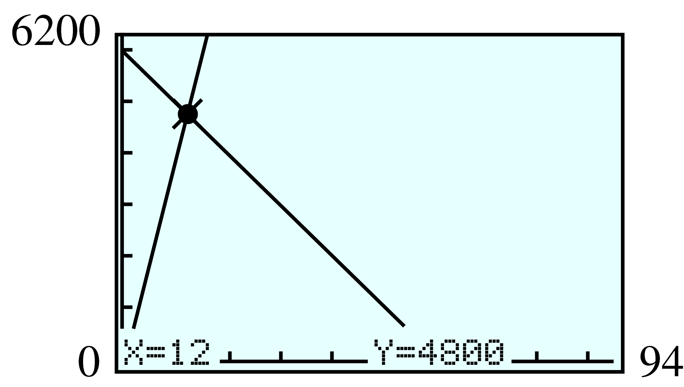
A woolens mill can produce \(400x\) yards of fine suit fabric if it can charge \(x\) dollars per yard. The mill’s clients in the garment industry will buy \(6000 - 100x\) yards of wool fabric at a price of \(x\) dollars per yard. Find the equilibrium price and the amount of fabric that will change hands at that price.
Solution.
Step 1.
We choose variables for the unknown quantities.
Price per yard:
\(x\)
Number of yards:
\(y\)
Step 2.
The supply equation tells us how many yards of fabric the mill will produce for a price of \(x\) dollars per yard.
\begin{equation*}
y=400x
\end{equation*}
The demand equation tells us how many yards of fabric the garment industry will buy at a price of \(x\) dollars per yard.
\begin{equation*}
y = 6000 - 100x
\end{equation*}
Step 3.
We graph the two equations on the same set of axes, as shown below. We set the window values to
Francine wants to join a health club and has narrowed it down to two choices. The Sportshaus charges an initiation fee of $500 and $10 per month. Fitness First has an initiation fee of $50 and charges $25 per month.
Let \(x\) stand for the number of months Francine uses the health club. Write equations for the total cost of each health club for \(x\) months.
Complete the table for the total cost of each club.
\(x\)
Sporthaus total cost
Fitness First total cost
6
12
18
24
30
36
42
48
Graph both equations on the grid.
When will the total cost of the two health clubs be equal?
14.
The Bread Alone Bakery has a daily overhead of $90. It costs $0.60 to bake each loaf of bread, and the bread sells for $1.50 per loaf.
Write an equation for the cost \(C\) in terms of the number of loaves, \(x\text{.}\)
Write an equation for the revenue \(R\) in terms of the number of loaves, \(x\text{.}\)
Graph the revenue, \(R\text{,}\) and cost, \(C\text{,}\) on the same set of axes. State the solution of the system.
How many loaves must the bakery sell to break even on a given day?
15.
The manager for Books for Cooks plans to spend $300 stocking a new diet cookbook. The paperback version costs her $5, and the hardback costs $10. She finds that she will sell three times as many paperbacks as hardbacks. How many of each should she buy?
Let \(x\) represent the number of hardbacks and \(y\) the number of paperbacks she should buy. Write an equation about the cost of the books.
Write a second equation about the number of each type of book.
Graph both equations and solve the system using the grid.
Answer the question in the problem.
16.
There were 42 passengers on a local airplane flight. First-class fare was $80, and coach fare was $64. If the revenue for the flight totaled $2880, how many first-class and how many coach passengers paid for the flight?
Write algebraic expressions to fill in the table.
Number of tickets
Cost per ticket
Revenue
First-class
\(x\)
Coach
\(y\)
Total
Write an equation about the number of tickets sold.
Write a second equation about the revenue from the tickets.
Graph both equations on graph paper and solve the system. (Hint: Find the intercepts of each equation to help you choose scales for the axes.)
Answer the question in the problem.
17.
Mel’s Pool Service can clean \(1.5x\) pools per week if it charges \(x\) dollars per pool, and the public will book \(120 - 2.5x\) pool cleanings at \(x\) dollars per pool.
Find the equilibrium price and the number of pools Mel will clean at that price.
18.
Explain how you can tell, without graphing, that the system has no solution.
\begin{gather*}
3x=y+3\\
6x-2y=12
\end{gather*}
Explain how you can tell, without graphing, that the system has infinitely many solutions.
\begin{gather*}
-x+2y=4\\
3x=6y-12
\end{gather*}
19.
According to the Bureau of the Census, the average age of the U.S. population is steadily rising. The table gives data for two types of average, the mean and the median, for the ages of women. (The "mean" is the familiar average, and the "median" is the middle age: half of all women are older and half younger than the median.)
Date
1990
1992
1994
1996
1998
Median age
\(34.0\)
\(34.6\)
\(35.2\)
\(35.8\)
\(36.4\)
Mean age
\(36.6\)
\(36.8\)
\(37.0\)
\(37.3\)
\(37.5\)
Which is growing more rapidly, the mean age or the median age?
Plot the data for median age versus the date, using 1990 as \(t=0\text{.}\) Draw a line through the data points.
What is the meaning of the slope of the line in part (b)?
Plot the data for mean age versus date on the same grid. Draw a line that fits the data.
Use your graph to estimate when the mean age and the median age were the same.
If the median age of women in the United States is greater than the mean age, what does this tell you about the population of women?
20.
The table below gives data for the mean and median ages for men in the United States. Repeat Problem 19 for these data.