Chapter 10 Logarithmic Functions
In Chapter 7 we used logarithms to solve exponential equations. Recall that a logarithm is really an exponent, so that, for example, \(\log_2 {(16)}\) means "what exponent on base 2 will give me 16?" The answer of course is 4, so \(\log_2 {(16)} = 4\text{.}\)
In this chapter, we consider functions defined in terms of logartihms, and logarithmic functions as models in their own right. A logarithmic function looks like \(f(x) = \log_b {(x)}\text{,}\) where \(b\) is the base and \(x\) is a positive number. In Chapter 7 we saw that the base 10 logarithms, or common logarithms, appeared in many applications. Now we will also study another base for exponential and logarithmic functions, the natural base \(e\text{,}\) which is the most useful base for most scientific applications.
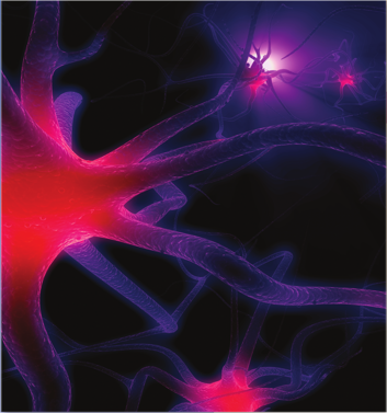
An interesting example of a logarithmic model arises in psychology. In 1885, the German philosopher Hermann Ebbinghaus conducted one of the first experiments on memory, using himself as a subject. He memorized lists of nonsense syllables and then tested his memory of the syllables at intervals ranging from 20 minutes to 31 days. After one hour, he remembered less than 50% of the items, but he found that the rate of forgetting leveled off over time. He modeled his data by the function
\begin{equation*}
y = \frac{184}{2.88 \log {(t)} + 1.84}
\end{equation*}
| Time elapsed | Percent remembered |
| \(20\) minutes | \(58.2\%\) |
| \(1\) hour | \(44.2\%\) |
| \(9\) hours | \(35.8\%\) |
| \(1\) day | \(33.7\%\) |
| \(2\) days | \(27.8\%\) |
| \(6\) days | \(25.4\%\) |
| \(31\) days | \(21.1\%\) |

Ebbinghaus’s model uses a logarithmic function. The graph of the data, shown above with \(t\) in minutes and \(y\) in percents, is called the "forgetting curve." Ebbinghaus’s work, including his application of the scientific method to his research, provides part of the foundation of modern psychology.
